Case Study 03 — Geophysical Feature Engineering

Seeing the Crust an AI Learns From

Raw gravity and magnetic grids look like weather maps — smooth blobs that hide the faults, intrusion margins and terrane sutures that actually control where ore forms. A handful of physics-based preprocessing filters — reduction-to-pole, derivatives, tilt and gradient transforms — convert those blobs into sharp, structure-revealing layers. On the Arabian Shield, known deposits are measurably enriched on the magnetic gradients these filters reveal — turning geology the eye can't see into candidate features an AI can weigh.

Geophysics Feature Engineering Mineral Targeting

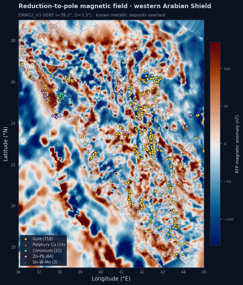
Request This Analysis Open Full Tutorial

Reduction-to-pole magnetic intensity of the Arabian Shield with 875 known metallic deposits overlaid — Reduction-to-pole magnetic field of the Arabian Shield (EMAG2_V3). Gold, copper, chromium and base-metal deposits cluster along the magnetic grain of the Neoproterozoic arc terranes.

875Known deposits analysed

1.5×Gradient enrichment at deposits

33Derived feature layers

4Commodity systems

Problem

The raw field is not the geology

Continental gravity and magnetic surveys are the cheapest window into the crust beneath cover — and the richest input to any data-driven prospectivity model. But the measured fields are deceptive. A magnetic anomaly is offset from the body that causes it (the field is dipolar and depends on magnetic latitude), and both gravity and magnetics blur deep regional sources together with the shallow structures that host ore. Fed to a model as-is, raw pixel values carry the right physics in the wrong frame.

The information an exploration AI actually needs is structural: where are the edges — the faults, the contacts, the buried intrusion margins, the terrane boundaries — and at what depth? That information is present in the data, but it is encoded in gradients and wavelengths, not in the raw amplitude. Preprocessing is how you decode it.

"A potential-field map answers a question no geologist asked: 'how strong is the field here?' Preprocessing rephrases it into the one they did: 'where is the structure?'"

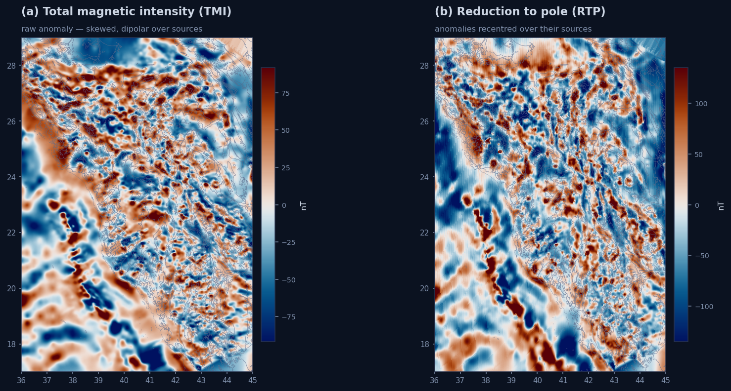
Raw total magnetic intensity versus reduction-to-pole — **Raw vs. reframed.** (a) Total magnetic intensity — anomalies are skewed and sit off their sources. (b) After reduction-to-pole, each anomaly is recentred over the body that causes it, so peaks line up with geology. Same data; a usable frame.

💡

Reduction-to-pole needs the ambient field direction. Here we use IGRF-14 at the survey epoch — inclination ≈ 39°, declination ≈ +3°, at the grid centre (the inclination falls toward the lower-latitude south-western shield). Get the angles wrong and the structures move.

Approach

A small suite of physics filters, each isolating one thing

Every filter in the suite is a closed-form operator in the Fourier domain — fast, deterministic and reproducible. Each one is designed to expose a single, interpretable aspect of the crust. Stacked together, they describe the structural architecture from several complementary angles.

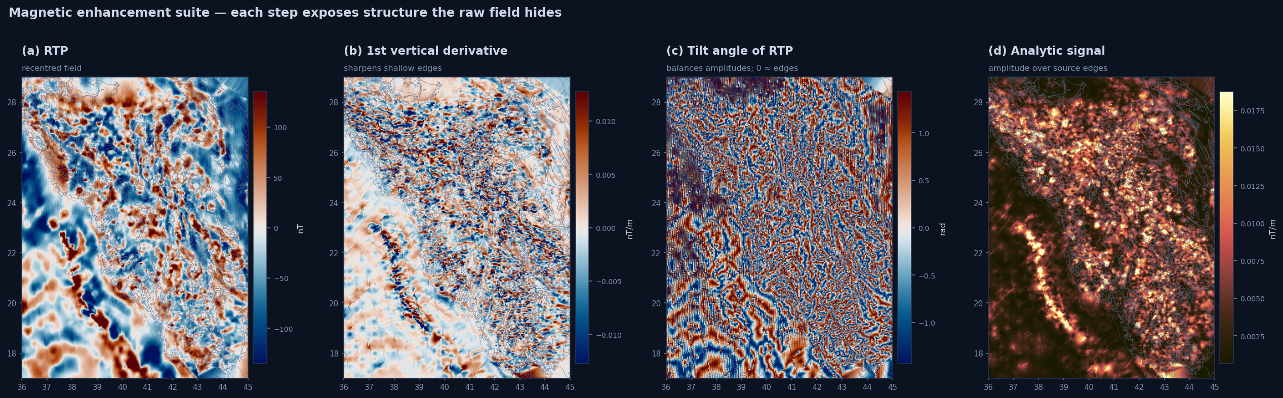
Magnetic enhancement suite: RTP, first vertical derivative, tilt angle, analytic signal — **The magnetic enhancement suite.** (a) Reduction-to-pole recentres the field. (b) The first vertical derivative sharpens shallow sources. (c) The tilt angle compresses amplitudes so weak and strong anomalies read alike — its zero contour traces source edges (strictly, over vertical contacts). (d) The analytic signal peaks close to the edges of magnetic bodies, largely independent of magnetisation direction (strictly so only in 2-D). Each is a different question asked of the same crust.

What each filter exposes

01
Reduction to pole: removes the magnetic-latitude skew so anomalies sit over their sources.
02
Vertical & horizontal derivatives: amplify short-wavelength, shallow structure and locate boundaries.
03
Tilt angle: a normalised derivative that equalises amplitudes — superb for mapping faint structures next to strong ones.
04
Analytic signal / total horizontal gradient: amplitude maxima sit close to the edges of bodies — direct contact mapping (the analytic signal is largely magnetisation-direction independent; the total horizontal gradient is not).
05
Upward continuation: tunes the depth of view, separating the deep regional field from shallow residual structure.

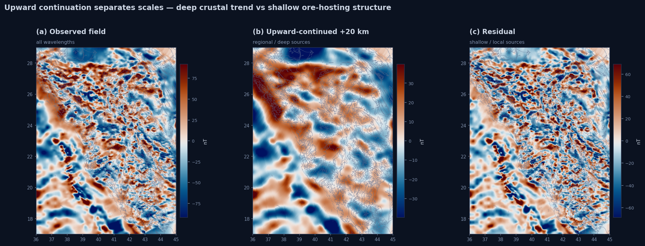
Upward continuation separates regional and residual fields — **Scale separation by upward continuation.** The observed field (a) is split into a deep regional trend (b, continued 20 km upward) and a shallow residual (c). Ore systems live in the residual; the regional sets the crustal stage.

⚙️

All nine magnetic and twenty-four gravity layers were produced with Geonome's open Kalpa Geophysics plugin (Fatiando harmonica back-end) — the same one-click filters an explorationist runs in the desktop app.

Why It Matters for AI

These filters are the features — and the deposits prove it

A modern prospectivity model does not ingest a magnetic map; it ingests a stack of features. The preprocessing suite is that stack. By converting amplitude into gradients, tilt and continuation bands, the filters express the field in the structural language a tree-based or neural model can split on — and they make the deposit-controlling signal explicit rather than buried.

The test is simple: do known deposits sit where the filters say the structure is? Across the western shield, the gold deposits are enriched on stronger gradients than random background — about two-thirds exceed the background-median gradient. That is an association, not a proven control — the deposits are spatially clustered and other factors are in play — but it is exactly the kind of statistical separation a model can exploit, and it is far stronger than for the raw field.

📈

A measurable association, not a mechanism. Separability is the point: a layer whose values differ between deposits and background is a layer a model can use. Whether that difference reflects a genuine geological control is a separate question, settled by validation — not by the histogram. Raw amplitude barely separates them; its gradients do.

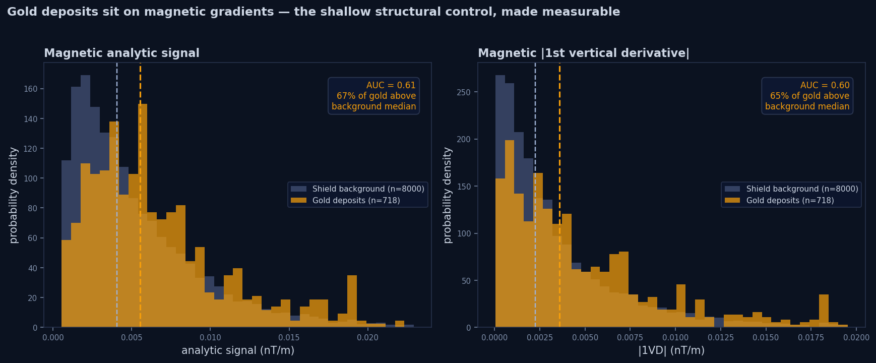
Deposits are enriched on magnetic gradients versus background — **Gold prefers the gradients.** Distribution of the magnetic analytic signal and |vertical derivative| at gold-deposit sites (orange) versus shield background (blue). Around two-thirds of deposits exceed the background median (AUC 0.61) — the structural control the eye senses, now quantified.

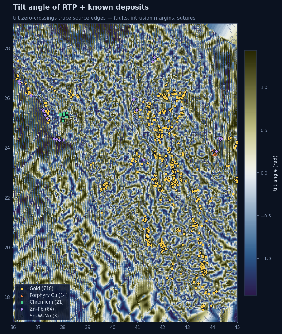
Tilt angle of the reduction-to-pole field with deposits overlaid — **Tilt-angle edges and the mineralised belts.** The tilt angle of the RTP field; its blue-to-red transitions mark source edges. The Nabitah suture, the Wadi Bidah VMS belt and the Wadi Tathlith gold belt thread along these magnetic discontinuities, which are commonly interpreted as crustal sutures and shear corridors — a striking association to test, not a proven control.

The Deep-Earth Layer — and a Caution

Gravity reads the deep crust — but read it carefully

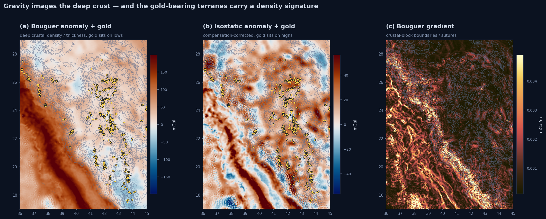
Where magnetics resolves shallow, ore-scale structure, gravity reaches deeper: the Bouguer and isostatic fields image the density and thickness of the crust — a regional context layer, complementary to the shallow magnetic edges.

It is tempting to go further. In our data the gold deposits do fall, more often than not, on Bouguer lows (71% below the background median) and isostatic highs (76% above). But this is exactly where geophysical interpretation gets dangerous — and a worked example of what not to claim. Two confounders dominate: the Bouguer field is −0.94 correlated with elevation, and the gold belts simply sit in the higher western shield, so "gold on Bouguer lows" is largely "gold at altitude". And the 718 deposits are not 718 independent samples — they cluster into roughly 15 belts (tens of independent cells), which inflates any naive statistic.

⚠️

Correlation is not control. Gravity earns its place as a deep-crustal context feature. Whether its apparent gold association is a real signal — rather than topography and clustering in disguise — is a hypothesis to be tested with elevation-controlled, spatially-blocked validation, not asserted from a histogram.

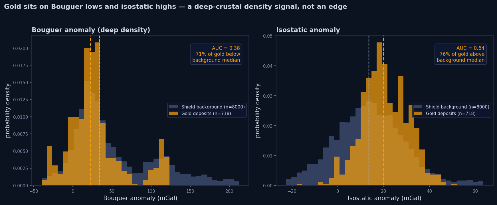
Apparent association of gold deposits with Bouguer lows and isostatic highs — **An apparent association — interpret with care.** Gold deposits (orange) vs shield background (blue) on the Bouguer and isostatic anomalies. The separation is real in this dataset, but largely explained by topography (Bouguer ≈ −0.94 with elevation) and by belt clustering — so it is a cautionary example, not a demonstrated deep-crustal control.

Gravity suite: Bouguer and isostatic anomalies with gold, and Bouguer gradient — **Gravity images the deep crust.** (a) Bouguer anomaly and (b) isostatic anomaly with gold deposits overlaid; (c) the Bouguer gradient outlines the boundaries between crustal blocks. What gravity reliably gives the feature stack is regional crustal *context* — the deposit co-location in (a)–(b) should be read with the caveats above, not as a genetic signal.

Technology Stack

Open data, reproducible filters, audit-ready features

Every layer in this study is reproducible from open data with open filters — no black boxes between the satellite-era field and the model-ready feature. The same preprocessing runs inside the Kalpa desktop app and in headless notebooks, so a feature stack built for a research demo is the one that ships to production.

EMAG2_V3 WGM2012 Reduction to Pole Tilt / THG Analytic Signal Upward Continuation harmonica Kalpa Geophysics IGRF-14 GeoTIFF Output

Inputs are the public EMAG2_V3 magnetic and WGM2012 gravity compilations, cropped to the Arabian Shield and filtered with Geonome's Kalpa Geophysics plugin. Each output is a georeferenced GeoTIFF aligned cell-for-cell with the others — drop-in features for the prospectivity pipeline, openable in QGIS, ArcGIS or Leapfrog.

The result is a feature stack whose every band has a one-line physical meaning, so your geological team can audit why a target scores — the structural reason traces straight back to a filter and a field.

References

Sources & further reading

The methods, datasets and geology in this case study are documented in the peer-reviewed and agency literature below. Every entry was verified against a resolving DOI or the issuing agency; the full technical treatment is in the tutorial.

Show full reference list

Potential-field theory & filters

Baranov, V. (1957). A new method for interpretation of aeromagnetic maps: pseudo-gravimetric anomalies. Geophysics, 22(2), 359–382. doi:10.1190/1.1438369
Baranov, V., & Naudy, H. (1964). Numerical calculation of the formula of reduction to the magnetic pole. Geophysics, 29(1), 67–79. doi:10.1190/1.1439334
Blakely, R. J. (1995). Potential Theory in Gravity and Magnetic Applications. Cambridge University Press. doi:10.1017/CBO9780511549816
Gunn, P. J. (1975). Linear transformations of gravity and magnetic fields. Geophysical Prospecting, 23(2), 300–312. doi:10.1111/j.1365-2478.1975.tb01530.x
Henderson, R. G., & Zietz, I. (1949). The computation of second vertical derivatives of geomagnetic fields. Geophysics, 14(4), 508–516. doi:10.1190/1.1437558
Jacobsen, B. H. (1987). A case for upward continuation as a standard separation filter for potential-field maps. Geophysics, 52(8), 1138–1148. doi:10.1190/1.1442378
Cordell, L. (1979). Gravimetric expression of graben faulting in Santa Fe country and the Española Basin, New Mexico. New Mexico Geological Society Guidebook, 30, 59–64. doi:10.56577/FFC-30.59
Cordell, L., & Grauch, V. J. S. (1985). Mapping basement magnetization zones from aeromagnetic data in the San Juan basin, New Mexico. In W. J. Hinze (Ed.), The Utility of Regional Gravity and Magnetic Anomaly Maps (pp. 181–197). SEG. doi:10.1190/1.0931830346.ch16
Blakely, R. J., & Simpson, R. W. (1986). Approximating edges of source bodies from magnetic or gravity anomalies. Geophysics, 51(7), 1494–1498. doi:10.1190/1.1442197
Nabighian, M. N. (1972). The analytic signal of two-dimensional magnetic bodies with polygonal cross-section. Geophysics, 37(3), 507–517. doi:10.1190/1.1440276
Nabighian, M. N. (1984). Toward a three-dimensional automatic interpretation of potential field data via generalized Hilbert transforms. Geophysics, 49(6), 780–786. doi:10.1190/1.1441706
Roest, W. R., Verhoef, J., & Pilkington, M. (1992). Magnetic interpretation using the 3-D analytic signal. Geophysics, 57(1), 116–125. doi:10.1190/1.1443174
Li, X. (2006). Understanding 3D analytic signal amplitude. Geophysics, 71(2), L13–L16. doi:10.1190/1.2184367
Miller, H. G., & Singh, V. (1994). Potential field tilt—a new concept for location of potential field sources. Journal of Applied Geophysics, 32(2–3), 213–217. doi:10.1016/0926-9851(94)90022-1
Verduzco, B., Fairhead, J. D., Green, C. M., & MacKenzie, C. (2004). New insights into magnetic derivatives for structural mapping. The Leading Edge, 23(2), 116–119. doi:10.1190/1.1651454
Salem, A., Williams, S., Fairhead, J. D., Ravat, D., & Smith, R. (2007). Tilt-depth method. The Leading Edge, 26(12), 1502–1505. doi:10.1190/1.2821934
Mendonça, C. A., & Silva, J. B. C. (1993). A stable truncated series approximation of the reduction-to-the-pole operator. Geophysics, 58(8), 1084–1090. doi:10.1190/1.1443492
Li, X. (2008). Magnetic reduction-to-the-pole at low latitudes: observations and considerations. The Leading Edge, 27(8), 990–1002. doi:10.1190/1.2967550
Clark, D. A., & Emerson, D. W. (1991). Notes on rock magnetization characteristics in applied geophysical studies. Exploration Geophysics, 22(3), 547–555. doi:10.1071/EG991547

Gravity & geodesy

Hinze, W. J., von Frese, R. R. B., & Saad, A. H. (2013). Gravity and Magnetic Exploration. Cambridge University Press. ISBN 978-0-521-87101-3.
Hackney, R. I., & Featherstone, W. E. (2003). Geodetic versus geophysical perspectives of the "gravity anomaly". Geophysical Journal International, 154(1), 35–43. doi:10.1046/j.1365-246X.2003.01941.x
Hinze, W. J., et al. (2005). New standards for reducing gravity data: the North American gravity database. Geophysics, 70(4), J25–J32. doi:10.1190/1.1988183
Li, X., & Götze, H.-J. (2001). Ellipsoid, geoid, gravity, geodesy, and geophysics. Geophysics, 66(6), 1660–1668. doi:10.1190/1.1487109
Simpson, R. W., Jachens, R. C., Blakely, R. J., & Saltus, R. W. (1986). A new isostatic residual gravity map of the conterminous United States. Journal of Geophysical Research, 91(B8), 8348–8372. doi:10.1029/JB091iB08p08348

Datasets & software

Maus, S., et al. (2009). EMAG2: a 2-arc min resolution Earth Magnetic Anomaly Grid. Geochemistry, Geophysics, Geosystems, 10(8), Q08005. doi:10.1029/2009GC002471
Meyer, B., Saltus, R., & Chulliat, A. (2017). Derivation and error analysis of EMAG2v3. Geochemistry, Geophysics, Geosystems, 18(12), 4522–4537. doi:10.1002/2017GC007280 · Data: NOAA NCEI, doi:10.7289/V5H70CVX
Balmino, G., Vales, N., Bonvalot, S., & Briais, A. (2012). Spherical harmonic modelling to ultra-high degree of Bouguer and isostatic anomalies. Journal of Geodesy, 86(7), 499–520. doi:10.1007/s00190-011-0533-4
Bonvalot, S., et al. (2012). World Gravity Map (WGM2012). BGI/CGMW/CNES/IRD. doi:10.18168/bgi.23
Alken, P., et al. (2021). International Geomagnetic Reference Field: the thirteenth generation. Earth, Planets and Space, 73, 49. doi:10.1186/s40623-020-01288-x
IAGA Working Group V-MOD (2024). International Geomagnetic Reference Field, 14th generation (IGRF-14) [Data set]. Zenodo. doi:10.5281/zenodo.14012303
Uieda, L., & the Fatiando a Terra developers (2024). Harmonica: forward modeling, inversion, and processing gravity and magnetic data [Software]. Zenodo. doi:10.5281/zenodo.3628741
Abdelrahman, K., et al. (2024). Structural mapping of the west central Arabian Shield using downward continued magnetic data. Journal of King Saud University – Science, 36(2), 103039. doi:10.1016/j.jksus.2023.103039

Arabian Shield geology & deposits

Stern, R. J. (1994). Arc assembly and continental collision in the Neoproterozoic East African Orogen. Annual Review of Earth and Planetary Sciences, 22, 319–351. doi:10.1146/annurev.ea.22.050194.001535
Johnson, P. R., et al. (2011). Late Cryogenian–Ediacaran history of the Arabian–Nubian Shield. Journal of African Earth Sciences, 61(3), 167–232. doi:10.1016/j.jafrearsci.2011.07.003
Stern, R. J., Johnson, P. R., Kröner, A., & Yibas, B. (2004). Neoproterozoic ophiolites of the Arabian–Nubian Shield. In T. M. Kusky (Ed.), Precambrian Ophiolites and Related Rocks (pp. 95–128). Elsevier. doi:10.1016/S0166-2635(04)13003-X
Johnson, P. R., Abdelsalam, M. G., & Stern, R. J. (2003). The Bi'r Umq–Nakasib suture zone in the Arabian–Nubian Shield. Gondwana Research, 6(3), 523–530. doi:10.1016/S1342-937X(05)71003-0
Stoeser, D. B., & Camp, V. E. (1985). Pan-African microplate accretion of the Arabian Shield. GSA Bulletin, 96(7), 817–826. doi:10.1130/0016-7606(1985)96<817:PMAOTA>2.0.CO;2
Worl, R. G. (1979). The Jabal Ishmas–Wadi Tathlith gold belt, Kingdom of Saudi Arabia (USGS Open-File Report 79-1519). doi:10.3133/ofr791519
Volesky, J. C., Stern, R. J., & Johnson, P. R. (2003). Geological control of massive sulfide mineralization in the Neoproterozoic Wadi Bidah shear zone. Precambrian Research, 123(2–4), 235–247. doi:10.1016/S0301-9268(03)00070-6
Abu-Alam, T. S., Abd El Monsef, M., & Grosch, E. (2019). Shear-zone hosted gold mineralization of the Arabian–Nubian Shield. Geological Society, London, Special Publications, 478, 287–307. doi:10.1144/SP478.13

Machine learning & statistical methodology

Bonham-Carter, G. F. (1994). Geographic Information Systems for Geoscientists: Modelling with GIS. Pergamon. ISBN 0-08-041867-8.
Carranza, E. J. M. (2008). Geochemical Anomaly and Mineral Prospectivity Mapping in GIS. Elsevier. ISBN 978-0-444-51325-0.
Rodriguez-Galiano, V., et al. (2015). Machine learning predictive models for mineral prospectivity. Ore Geology Reviews, 71, 804–818. doi:10.1016/j.oregeorev.2015.01.001
Zuo, R. (2020). Geodata science-based mineral prospectivity mapping: a review. Natural Resources Research, 29(6), 3415–3424. doi:10.1007/s11053-020-09700-9
Domingos, P. (2012). A few useful things to know about machine learning. Communications of the ACM, 55(10), 78–87. doi:10.1145/2347736.2347755
Roberts, D. R., et al. (2017). Cross-validation strategies for data with temporal, spatial, hierarchical, or phylogenetic structure. Ecography, 40(8), 913–929. doi:10.1111/ecog.02881
Ploton, P., et al. (2020). Spatial validation reveals poor predictive performance of large-scale ecological mapping models. Nature Communications, 11, 4540. doi:10.1038/s41467-020-18321-y
Meyer, H., & Pebesma, E. (2022). Machine learning-based global maps of ecological variables and the challenge of assessing them. Nature Communications, 13, 2208. doi:10.1038/s41467-022-29838-9
Hurlbert, S. H. (1984). Pseudoreplication and the design of ecological field experiments. Ecological Monographs, 54(2), 187–211. doi:10.2307/1942661
Hanley, J. A., & McNeil, B. J. (1982). The meaning and use of the area under a receiver operating characteristic (ROC) curve. Radiology, 143(1), 29–36. doi:10.1148/radiology.143.1.7063747
Hosmer, D. W., Lemeshow, S., & Sturdivant, R. X. (2013). Applied Logistic Regression (3rd ed.). Wiley. doi:10.1002/9781118548387

Go deeper — the full technical tutorial

Why potential fields need reframing, the maths of RTP and the derivative/tilt/gradient operators, scale separation by upward continuation, the gravity crustal frame, and how to turn the whole suite into a model-ready feature stack — with worked Arabian Shield figures throughout.

Open Full Tutorial