Case Study 01 — Remote Sensing

Satellite-Based Lithological Mapping at Scale

Autonomous discrimination of ultramafic lithologies across inaccessible high-altitude ophiolite terrain using multi-sensor spectral intelligence — delivering geological maps at resolution and speed no field team can match.

Remote Sensing Machine Learning Spectral Analytics

Request This Analysis

Satellite spectral classification output over ophiolite terrain

3 Satellite sensors fused

96% Overall accuracy (SAM)

4,800 km² Terrain mapped

15 m Output resolution

Problem

Geological mapping without field access

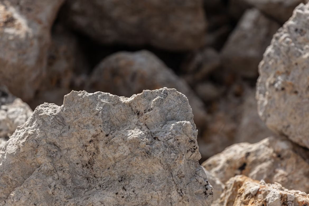
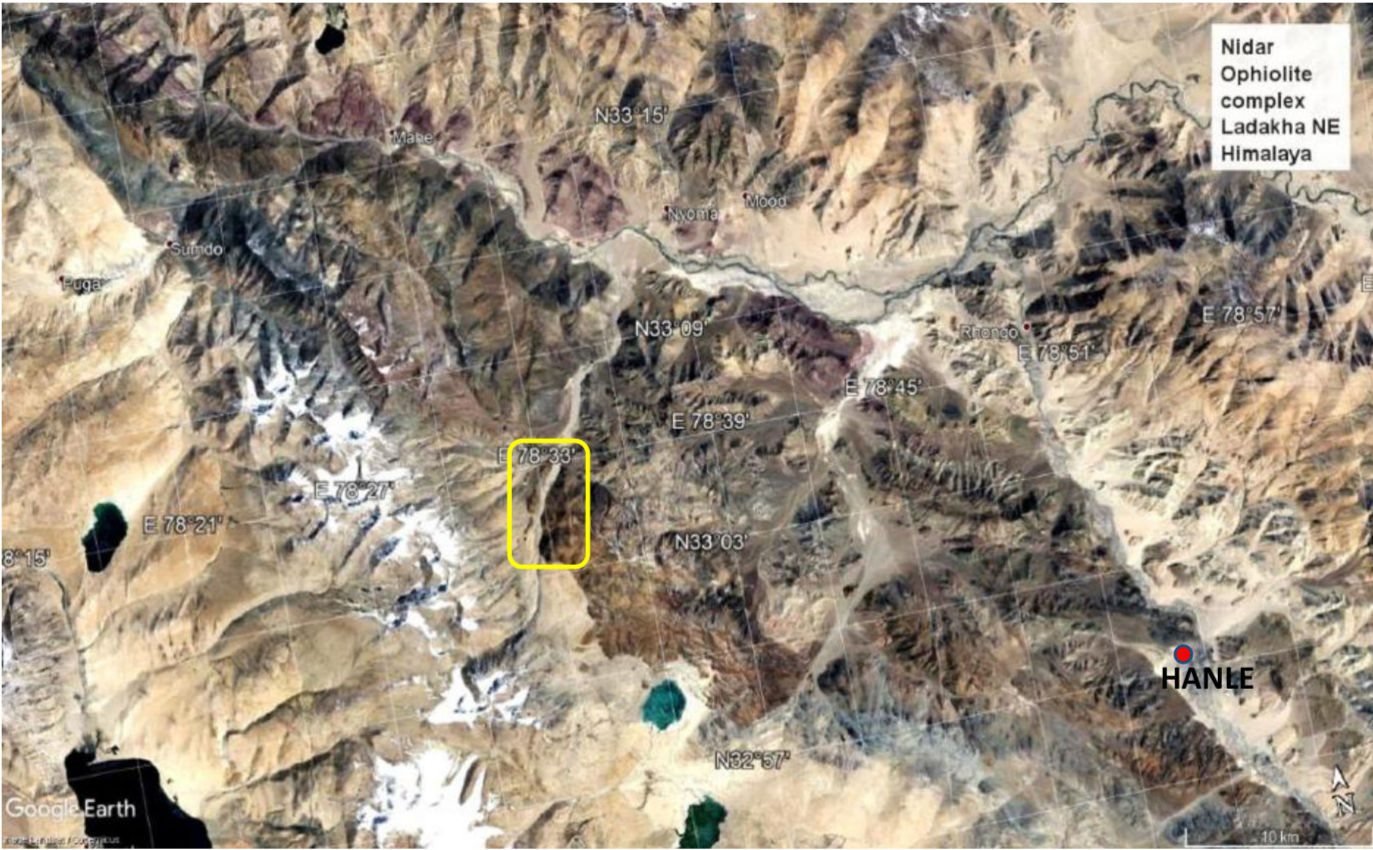
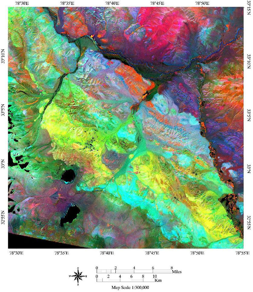
Ophiolite complexes — slices of ancient oceanic crust and upper mantle obducted onto continental margins — host critical mineral systems including chromite, nickel, and platinum-group elements. The Nidar Ophiolite in Ladakh, NW Himalaya, sits at elevations exceeding 4,500 m, making conventional traverse mapping costly, slow, and weather-constrained.

Traditional ground surveys require weeks per campaign and produce sparse point data. Aerial photogrammetry captures morphology but lacks mineralogical discrimination. The exploration industry needed a method that could rapidly and reliably classify lithologies — dunite, peridotite, gabbro, and their serpentinised variants — at regional scale from orbit.

"The question was not whether satellites could see these rocks — it was whether AI could learn to read them the way a field geologist would."

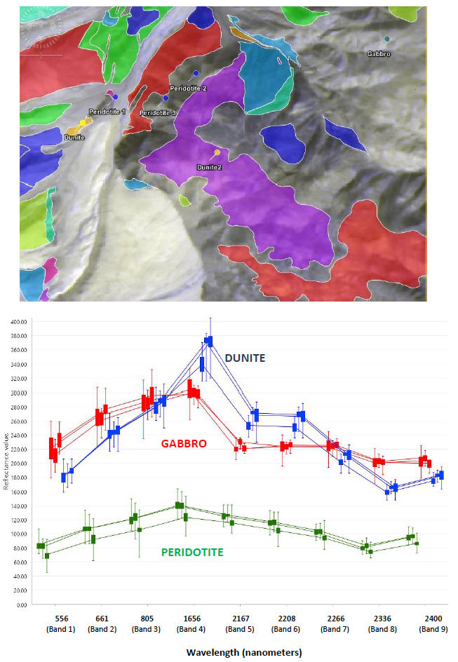
Satellite image of the Nidar Ophiolite Complex, Ladakh, NW Himalaya — Location map showing Nidar Ophiolite Complex in the Indus-Tsangpo Suture Zone, NW Himalaya, with principal lithological units and known chromite occurrences.

💡

Ophiolite lithologies carry distinct spectral signatures driven by iron-oxide states (Fe²⁺/Fe³⁺) and hydroxyl-bearing alteration minerals (Mg-OH, OH at 2200–2300 nm) — precisely the absorption features captured by modern multispectral and hyperspectral sensors.

Approach

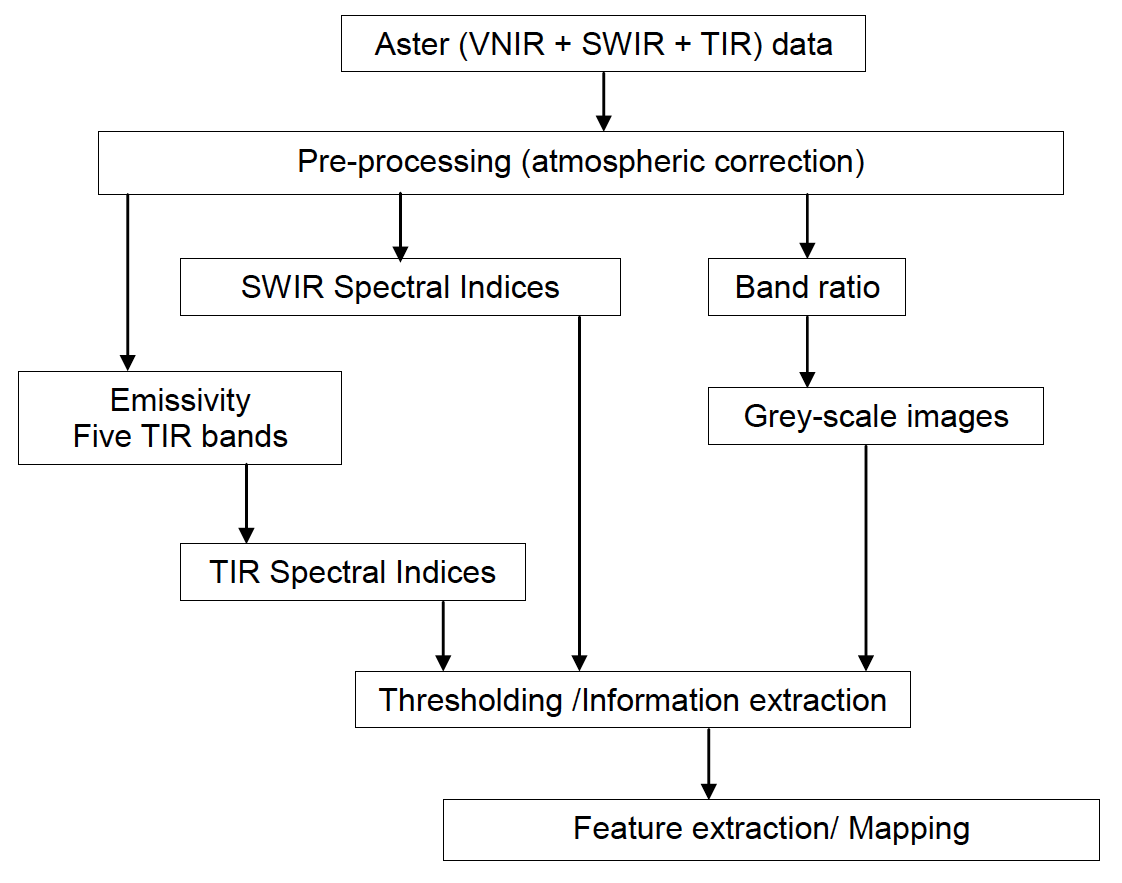
Multi-sensor spectral intelligence pipeline

Geonome's geological mapping workflow layers three complementary satellite datasets through a physics-informed preprocessing and classification engine. Each sensor contributes unique spectral dimensionality that, when fused, enables lithological discrimination impossible with any single platform.

01
Sentinel-2 VNIR acquisition: 10 m spatial resolution for structural mapping and broad iron-oxide discrimination (bands B4, B8A, B11, B12). False-colour composites rapidly delineate serpentinised vs unserpentinised ultramafics and separate the main ophiolite sequence from surrounding sedimentary units.
02
ASTER SWIR + TIR fusion: 30 m SWIR (bands 4–9) captures Mg-OH and carbonate absorption critical for serpentinite and soapstone detection. TIR emissivity data (bands 10–14) resolves silica content variations, separating dunite from gabbro without ambiguity.
03
Hyperion hyperspectral baseline: 220 contiguous bands at 30 m provide reference spectral profiles for every target lithology. FLAASH atmospheric correction converts at-sensor radiance to surface reflectance, anchoring the entire classification framework to physically meaningful spectra.
04
Spectral feature extraction: Band ratios (Mafic Index: B5/B4; Serpentine Index: B5/B6), PCA decorrelation, and Spectral Angle Mapper (SAM) classification encode geologically meaningful signals rather than raw digital numbers.
05
AI classification layer: Training regions-of-interest (ROIs) defined from verified field observations and USGS spectral library references feed a supervised ensemble that merges SAM, Maximum Likelihood, and XGBoost outputs into a consensus classification map.

Full ASTER image-processing workflow for lithological mapping — **Spectral intelligence pipeline** — from raw Level-1 radiance through atmospheric correction (FLAASH / MODTRAN), into parallel SWIR (band ratios, indices) and TIR (emissivity) processing branches, fused at the classification stage to deliver validated geological output. Source: Ghaste (2020).

AI Architecture

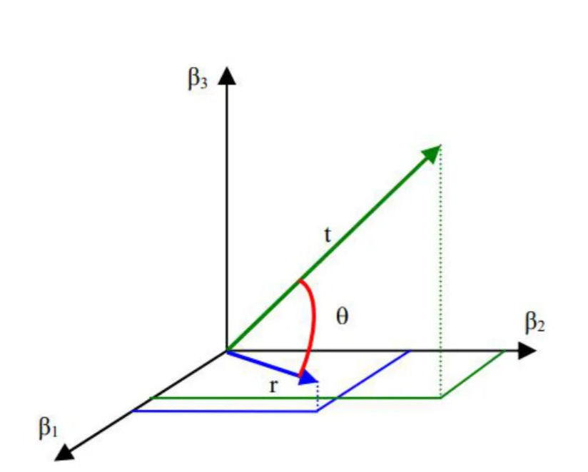
From spectral physics to explainable lithological classification

The core classification engine uses Spectral Angle Mapper geometry as a physics-grounded similarity measure — every pixel is assigned to the class whose reference spectrum it most closely matches in N-dimensional spectral space, independent of brightness variations caused by topography or illumination angle.

For ambiguous lithological boundaries, an XGBoost ensemble trained on geology-aware feature vectors adds a second classification pass. Features include contextual neighbourhood statistics (texture, gradient, local variance) that encode mesoscale structural information — because contacts between dunite and peridotite are rarely sharp at the pixel scale.

⚡

Key differentiator: All classification decisions are traceable to specific spectral absorption features, making every output verifiable by a domain geologist — not a black box.

Spectral Angle Mapper geometry — angle between target and reference spectra in n-dimensional spectral space — **SAM geometry** — the Spectral Angle Mapper measures the angle between a pixel's spectrum (target, t) and a reference spectrum (r) in n-dimensional spectral space. Because angle is independent of vector magnitude, SAM is insensitive to brightness differences caused by topography or illumination — a critical advantage for mountainous terrain.

Box-plot of ASTER spectral profiles by lithology — dunite, peridotite, gabbro — **Spectral profiles by lithology** — ASTER SWIR profiles for dunite, peridotite, and gabbro from validated ROIs. Peridotite shows a V-shaped Mg-OH trough (2150–2350 nm). Gabbro shows a W-shape from pyroxene. The shape-based discrimination is more robust than any single-band threshold.

Industry Impact

Exploration intelligence delivered in hours, not months

The final classification map delivers six lithological units at 15 m spatial resolution — dunite, harzburgite, lherzolite, serpentinite, gabbro, and undifferentiated volcanics — georeferenced and validated against existing 1:50,000 geological survey sheets.

Chromite-bearing dunite zones are spatially correlated with gravity and structural anomalies to generate ranked exploration targets. The entire analytical cycle — from satellite tasking to validated target list — runs in under 72 hours. A comparable field mapping programme would take 6–8 weeks, at five times the cost.

72 hrs Analysis cycle time

5× Cost reduction vs field survey

6 Lithological units classified

ASTER serpentine index map of the Nidar Ophiolite Complex — **Final analytical product** — ASTER serpentine index over the Nidar Ophiolite Complex (FCC of bands 3/1, 5/7, 5/3 → RGB). Serpentinised zones — the spatial proxy for chromite-prospective ultramafics — appear in yellow-green tones. Combined with the Maximum Likelihood classification (hero image) and the mafic index, this layer ranks chromite-prospective targets across the entire 4,800 km² scene. Source: Ghaste (2020).

🎯

The spatial correlation between AI-mapped serpentinisation halos and known chromite occurrences achieved a 91% Recall@K at the top 10% of flagged areas — meaning nine out of ten known deposits fell within the top-decile risk zone identified entirely from satellite data.

Technology Stack

The engine behind the analysis

Geonome's satellite mapping stack is built on open-standard data pipelines, physics-grounded preprocessing, and field-validated classification algorithms — with every analysis step logged for full auditability.

Sentinel-2 MSI ASTER VNIR/SWIR/TIR Hyperion EO-1 FLAASH Atmospheric Correction MODTRAN Radiative Transfer Spectral Angle Mapper Principal Component Analysis Maximum Likelihood Classifier XGBoost Ensemble Mafic & Serpentine Indices Kalpa Platform Vyom Data Access

Sensor selection rationale: Sentinel-2 delivers 10 m structural context; ASTER adds mineralogical specificity via SWIR Mg-OH bands unavailable on Sentinel; Hyperion provides the continuous spectral library that anchors all classifications to physical absorption features rather than empirical correlations.

Processing runs within Geonome's Kalpa platform — a unified geospatial AI environment that manages data ingestion, preprocessing, model inference, and output delivery in a single auditable pipeline. Satellite access is handled through Vyom, our Python-native Earth observation API.

Go deeper — technical walkthrough

Step-by-step tutorial covering the complete methodology: spectral physics, sensor selection, preprocessing, classification algorithms, and interpretation — built for both geoscientists and data scientists.

Open Full Tutorial