Raw Fields → Structural Filters → Model-Ready Features
Geophysical Preprocessing for AI Mineral Prospectivity
Before an AI can rank where to drill, it has to be shown the crust in a language it can learn from. Gravity and magnetic surveys carry that information across whole continents and beneath cover — but the raw fields disguise it. This tutorial builds the bridge: the physics-based filters that turn a smooth potential-field map into sharp layers of faults, contacts and intrusion edges — the exact features a prospectivity model needs. We work it end-to-end on the Arabian Shield, and check every claim against 875 known deposits.
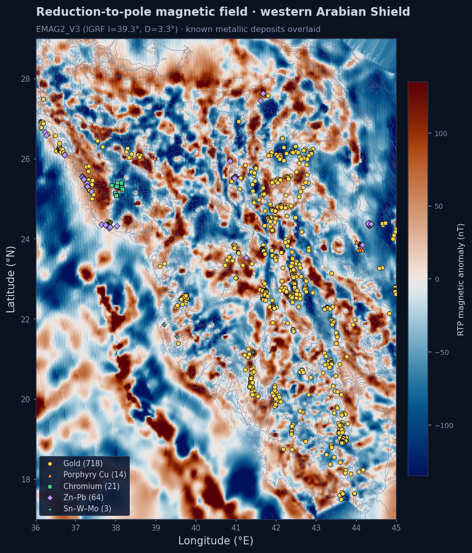
The destination: the reduction-to-pole magnetic field of the Arabian Shield with 875 known metallic deposits. Gold, copper, chromium and base-metal systems thread along the magnetic grain. By the end of this tutorial you will know exactly which filters reveal that grain — and why it makes the deposits learnable.
What Gravity and Magnetics Actually Measure
Two of the cheapest, most complete datasets in exploration are potential fields: the Earth's gravity and magnetic fields, mapped from satellites, aircraft and ground surveys. They are powerful precisely because they see through cover — but to use them well you must remember what each one responds to.
Magnetic field
Responds to the magnetic susceptibility of rocks — chiefly magnetite content. It lights up mafic/ultramafic bodies, banded iron, alteration that destroys or creates magnetite, and the faults that offset them. Sensitive to shallow, ore-scale structure.
Gravity field
Responds to density. The Bouguer anomaly images deep crustal density and thickness; its gradients outline the boundaries between crustal blocks. Sensitive to deep, regional architecture.
Geology / deposits
The ground truth. Surface maps and known occurrences tell you what the fields mean — and let you test whether a processed layer actually tracks mineralisation.
Why potential fields are a "field"
Both obey Laplace's equation in source-free space, which is what makes the whole filter toolkit possible: a potential field measured on one surface can be mathematically continued, differentiated, or re-pointed to a different magnetisation direction — all as exact operations in the Fourier (wavenumber) domain. Preprocessing is not cosmetic image enhancement; it is the physics of the field, applied.
Why the Raw Field Misleads
If you hand a raw magnetic grid to a machine-learning model, you are handing it the right physics in the wrong frame. Three properties of potential fields make the unprocessed amplitude a poor feature.
The anomaly is offset from its source
Because the magnetic field is dipolar and the Earth's field is inclined, a compact magnetic body does not produce a single peak over its centre — it produces a high–low couplet that is shifted and asymmetric. The brightest pixel is not above the rock. A model trained on raw amplitude learns a systematically displaced target.
Every wavelength is superimposed
A raw value sums the deep regional field and the shallow local field. The crustal-scale trend (hundreds of km) and the prospect-scale structure (a few km) arrive in the same number. Until you separate scales, the model cannot tell "thick crust" from "buried intrusion".
Amplitude hides faint structure
A strong iron-rich body can be a hundred times brighter than a subtle fault that actually controls ore. On a linear colour scale the fault is invisible. The information is there — in the shape of the field, not its magnitude — but raw amplitude buries it.
The preprocessing suite addresses each of these in turn: reduction-to-pole fixes the offset, upward continuation separates the scales, and the derivative/tilt family rescales the field so structure — not magnitude — dominates.
Reduction to Pole — Putting Anomalies Back Over Their Sources
Reduction-to-pole (RTP) mathematically transforms the field into what it would look like if it were measured at the magnetic pole, where the inducing field is vertical. The dipolar couplet collapses to a single anomaly centred on the body. It is the first step in almost every magnetic interpretation.
FRTP(k) = F(k) · |k|² / [ ( m̂·K )( f̂·K ) ] , K = ( i kx, i ky, |k| )
K is the complex 3-D wavevector; f̂ = ( cos I sin D, cos I cos D, sin I ) is the ambient-field direction and m̂ the magnetisation direction (I = inclination, D = declination). The denominator is a product of two complex factors — it collapses to a single squared factor only for purely induced magnetisation (m̂ = f̂). Equivalently, applied to the total-field anomaly, the per-azimuth factor is [ sin I + i cos I cos(D − θ) ]. The operator divides out the geometry of the inclined inducing field, so it needs the correct I and D for the survey's place and epoch (Baranov & Naudy, 1964; Gunn, 1975; Blakely, 1995).
For the Arabian Shield we evaluate the International Geomagnetic Reference Field (IGRF-14) at the grid centre for the survey epoch: inclination ≈ 39°, declination ≈ +3° (grid-centre values — the inclination falls toward the lower-latitude south-western shield, e.g. ≈ 33° in the west-central shield; Abdelrahman et al., 2024). Use the wrong angles and every anomaly shifts — and so does every "structure" a downstream model would key on.
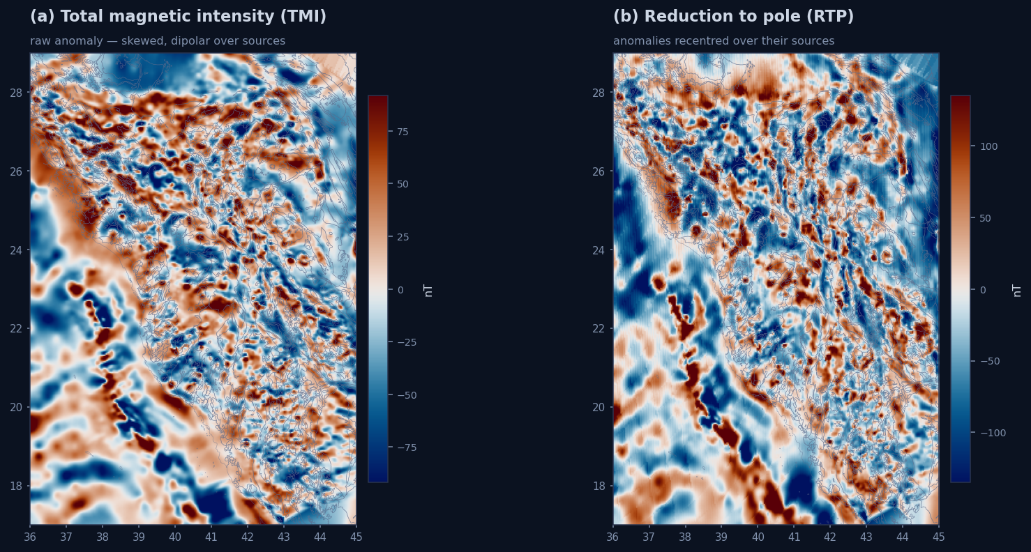
Figure 3.1 — (a) Raw total magnetic intensity (TMI): anomalies are skewed and sit off their sources. (b) After RTP, peaks recentre over the bodies that cause them and align with mapped geology. Identical data — only the frame has changed.
Key Insight
RTP is unstable at low magnetic latitudes (small |I|), where the operator blows up along one wavenumber direction. Near the magnetic equator you reduce-to-equator or apply a stabilised kernel instead. On the Arabian Shield, I ≈ 39° — comfortably stable — but the principle matters anywhere you process magnetics: always check the inclination before you trust an RTP.
Derivatives — Sharpening Structure
Differentiation is the workhorse of potential-field interpretation. Taking a derivative suppresses long-wavelength regional content and amplifies short-wavelength, shallow structure — exactly where ore-controlling faults and contacts live. In the Fourier domain it is a one-line operation.
∂nf/∂zn ⇌ |k|n · F(k) ∂f/∂x ⇌ i kx · F(k) ∂f/∂y ⇌ i ky · F(k)
The first vertical derivative (1VD) is the most-used: it acts as a high-pass filter that crisps up the edges of shallow sources and resolves anomalies that merge in the raw field. The horizontal derivatives ∂f/∂x and ∂f/∂y are the raw material for the gradient and tilt transforms that follow.
The catch — and why padding and detrending matter
Multiplying by |k|n amplifies high wavenumbers, which also amplifies noise and edge artefacts. Robust derivatives require the grid to be gap-free, evenly sampled, detrended and tapered before the FFT. The Kalpa plugin handles this automatically — it infills data gaps, removes a planar trend, and pads the grid — so the derivative reflects geology, not the survey boundary.
Total Gradient & Analytic Signal — Mapping Edges Directly
Derivatives sharpen structure but still depend on magnetisation direction. The gradient transforms combine them into quantities whose maxima sit directly over the edges of bodies — turning interpretation into edge-finding.
THG = √( (∂f/∂x)² + (∂f/∂y)² ) |AS| = √( (∂f/∂x)² + (∂f/∂y)² + (∂f/∂z)² )
The total horizontal gradient peaks over near-vertical contacts and faults — it is the classic boundary-mapper (though, like the derivatives, it remains magnetisation-direction dependent for magnetic data). The analytic signal adds the vertical derivative, giving a positive quantity that sits over source edges largely independently of the magnetisation direction — strictly so only in 2-D, and approximately in 3-D (Li, 2006) — which is why it is comparatively robust at low latitudes or where remanence is present. Both convert the field into a clean "where are the boundaries?" image.
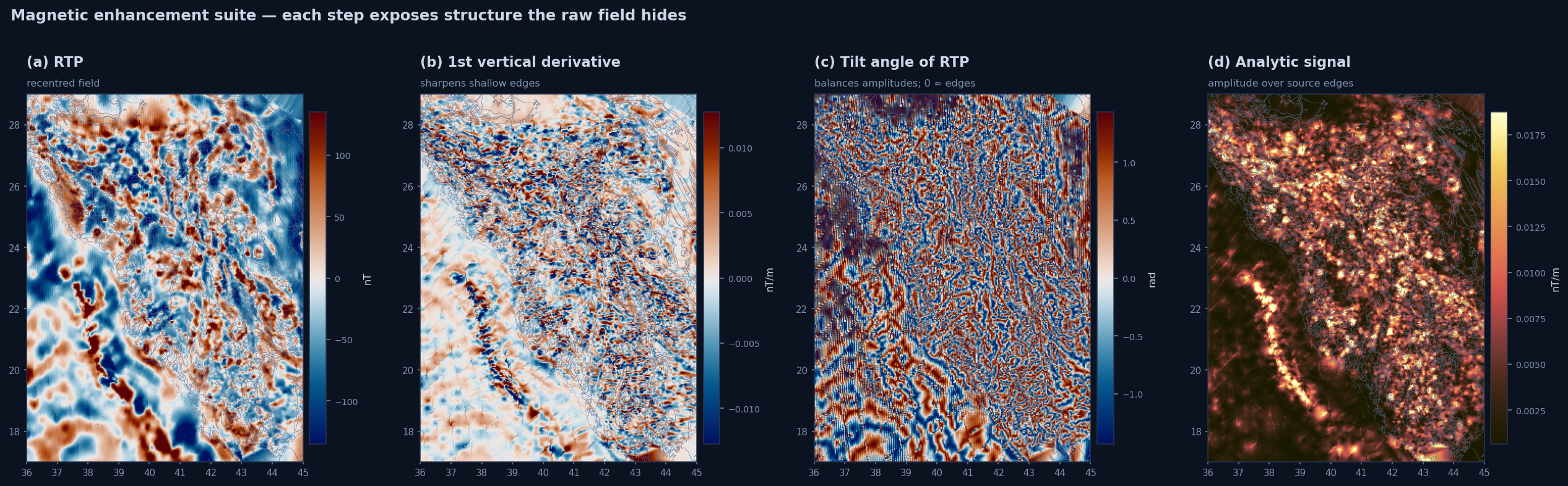
Figure 5.1 — The same magnetic field seen four ways. (a) RTP, (b) first vertical derivative, (c) tilt angle, (d) analytic signal. Moving left to right, amplitude gives way to structure: by panel (d), the image is essentially a map of magnetic boundaries — exactly the kind of layer a model can split on.
The Tilt Angle — Equalising Strong and Weak
The single most useful display transform for structure is the tilt angle. It normalises the vertical derivative by the horizontal gradient, so it depends on the shape of the field rather than its amplitude — faint anomalies over deep or weakly magnetic rocks read just as clearly as strong ones.
θ = arctan( (∂f/∂z) / √( (∂f/∂x)² + (∂f/∂y)² ) )
Bounded to ±90°. Positive over sources, negative off them, and θ = 0 over the edge (strictly, above a vertical contact; Salem et al., 2007) — so the zero contour is a near-automatic structure map.
Because arctan compresses the dynamic range, the tilt angle is the great equaliser: it makes the subtle
structural fabric of a whole terrane visible at once. Drag the slider below to watch the raw field dissolve into
pure structure.

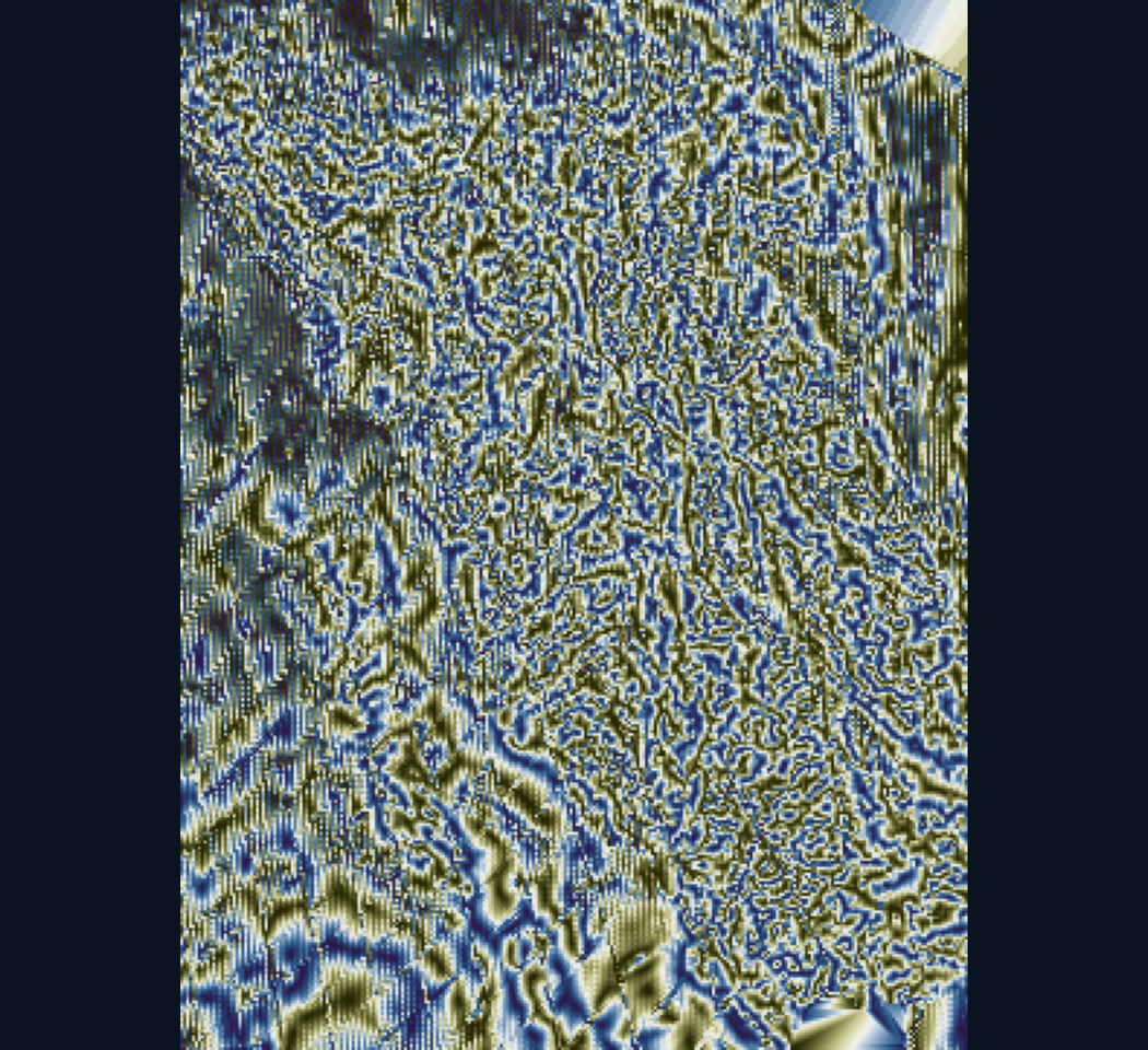
Figure 6.1 (interactive) — Drag across the image. Left of the handle: the raw magnetic intensity, dominated by a few bright bodies. Right: the tilt angle, where the entire structural grain of the shield — faults, contacts, fold trends — emerges at uniform contrast.
Why this matters for AI
A model splits on whatever separates deposits from background. On raw amplitude, a deep ore-controlling fault and barren bedrock can have nearly identical values — there is nothing to split on. On the tilt angle, the fault is a sharp zero-crossing and the bedrock is not. The transform doesn't add information; it moves the existing information into a form the model can act on.
Upward Continuation — Choosing Your Depth of View
Upward continuation recomputes the field as if it were measured at a higher altitude. Raising the observation level attenuates short wavelengths faster than long ones, so the continued field is a smoothed, deep-source-dominated version of the original. It is the cleanest way to separate the regional from the residual.
Fh(k) = F(k) · e−|k| h residual = f − fh
Continue the field up by, say, 20 km and you isolate the regional field of deep crustal sources. Subtract that from the observed field and you isolate the residual — the shallow structure where ore systems live. Feeding a model both the regional and several residual bands lets it reason about depth without ever being told what depth is.
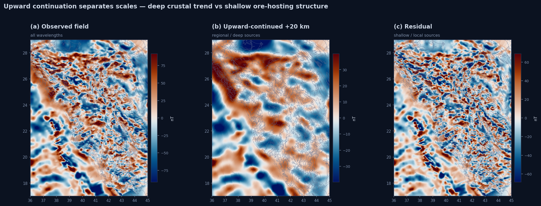
Figure 7.1 — (a) Observed field. (b) Upward-continued 20 km — the deep regional trend. (c) Residual — shallow, local structure. Each becomes a separate feature band; together they encode a crude depth dimension.
The Gravity Family — Bouguer, Free-Air, Isostatic, Disturbance
Gravity tells a different and complementary story: density, not magnetism. The same derivative, gradient and tilt operators apply — but there is no reduction-to-pole, because gravity's source is mass: a scalar, monopolar density distribution with no magnetisation or inducing-field direction to correct (unlike the dipolar magnetic field). Instead, the choice is which gravity anomaly to start from, each having removed a different reference effect.
Free-air
Corrected for the height variation of normal gravity (not for the rock mass below the station). Strongly tracks topography — useful, but dominated by terrain.
Bouguer
Also removes the gravitational pull of the rock above sea level. The workhorse for crustal density and thickness.
Isostatic
Further removes the deep root that compensates topography — sharpens mid-crustal density contrasts.
Disturbance
Observed minus normal gravity at the true station — a cleaner reference for many crustal studies.
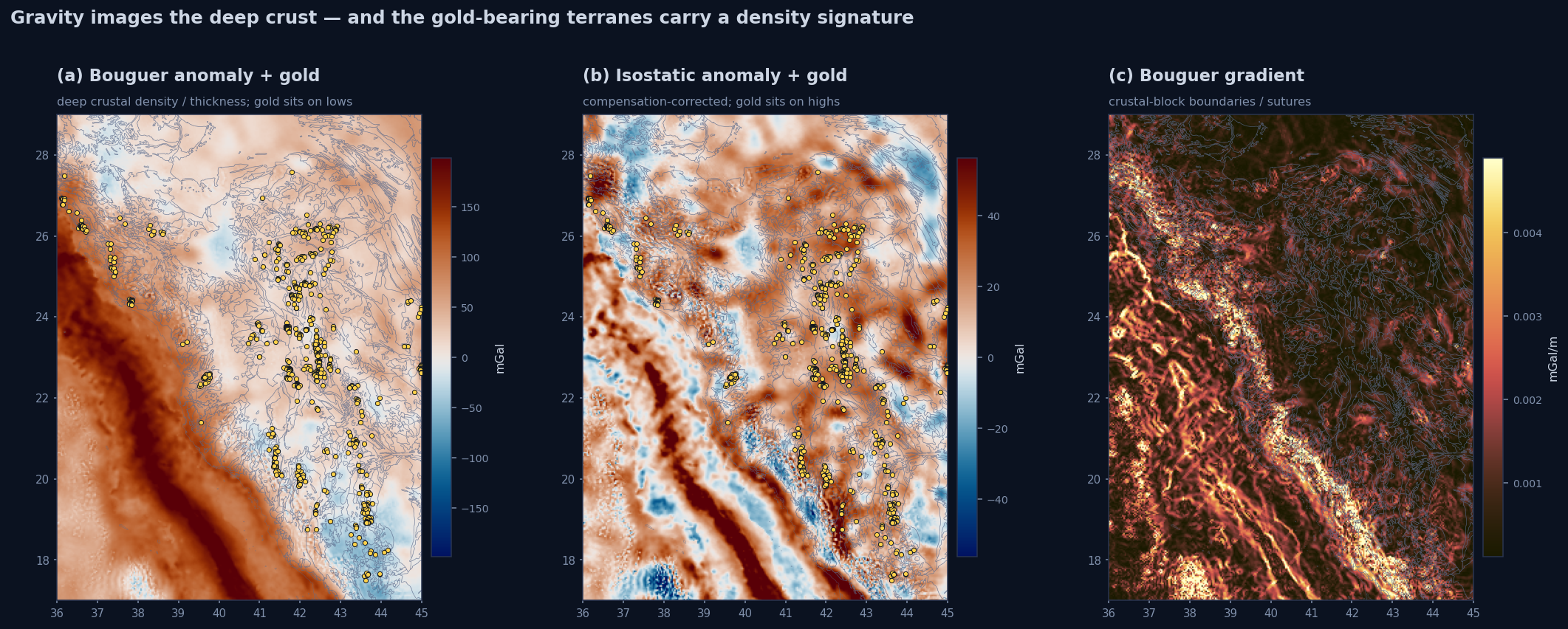
Figure 8.1 — Gravity preprocessing on the western Arabian Shield. (a) Bouguer anomaly and (b) isostatic anomaly with gold deposits overlaid — deep crustal density and thickness. (c) The Bouguer total horizontal gradient traces the boundaries between crustal blocks. The same operators as the magnetics, now applied to density.
Gravity Reads the Deep Crust — and a Lesson in Not Over-Reading It
Gravity's Bouguer and isostatic fields are a statement about density kilometres down — genuinely useful as a regional context layer. They also make a perfect teaching case for the most important discipline in this whole subject: telling a real signal from a confounded one.
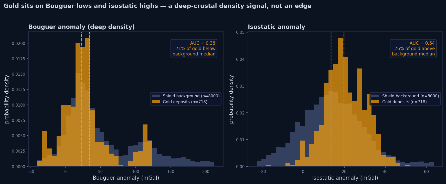
Figure 9.1 — Gold deposits (orange) vs shield background (blue) on the Bouguer and isostatic anomalies. Gold appears to concentrate on Bouguer lows (71% below the background median) and isostatic highs (76% above). A tempting "deep-crustal gold signature" — but look closer before believing it.
Why this is mostly an artefact — and how to catch it
Two checks deflate the story. (1) A confounder: the Bouguer anomaly is −0.94 correlated with elevation, and the gold belts sit in the higher western shield (median 949 m vs 805 m for background). So "gold on Bouguer lows" is largely "gold at altitude" — isostasy, not ore-bearing crust. (2) Pseudo-replication: the 718 gold points are not independent — they cluster into ~15 belts (tens of effective cells), so a naive AUC or percentage is badly over-confident. The honest verdict: gravity is a sound deep-crustal context feature, but its apparent gold association is not demonstrated — it must be tested with elevation-controlled, spatially-blocked validation.
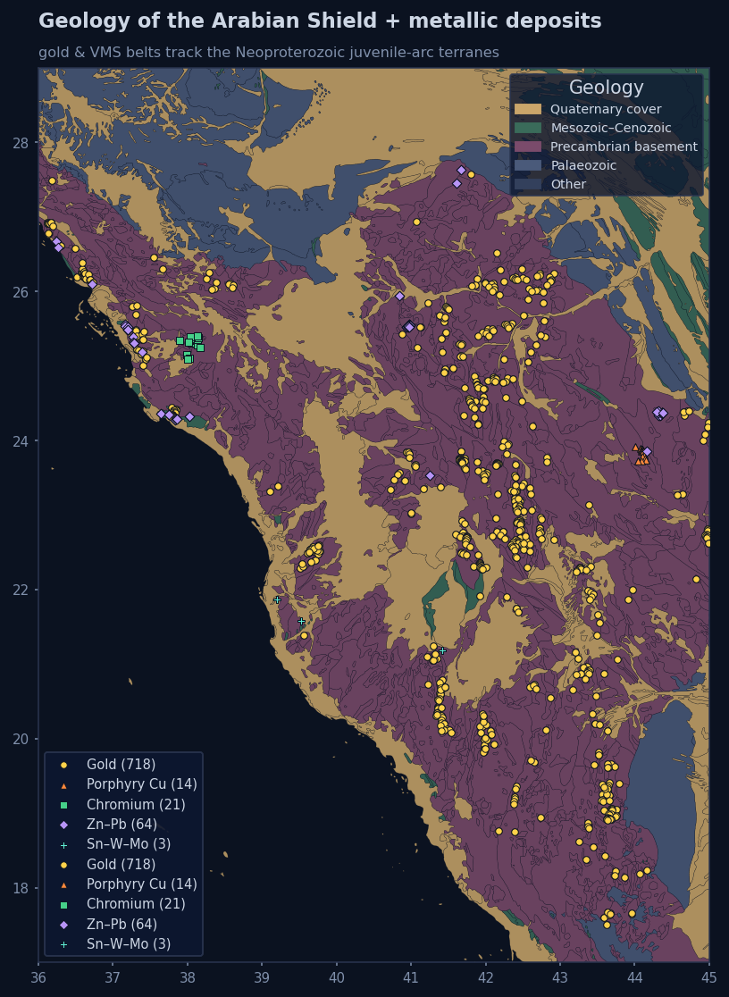
Figure 9.2 — Surface geology with the deposits by commodity. The gold and VMS belts sit inside the Precambrian juvenile-arc terranes — useful ground truth, and a reminder that the deposits are clustered by geology, which is exactly why per-point geophysical statistics must be declustered before they are trusted.
Building the Feature Stack
A prospectivity model never sees a "map". It sees, at every grid cell, a vector of numbers — the feature stack. The preprocessing suite is precisely how that vector is built: each filter contributes one or more bands, each with a one-line physical meaning.
Figure 10.1 — From three open datasets to one feature vector per cell. Magnetics contributes shallow-structure bands; gravity the crustal frame; geology the lithological context. Neighbourhood statistics add regional context. This stack — not the raw maps — is what the model in Tutorial 2 learns from.
The feature-engineering principle
The choice of algorithm matters far less than the choice of representation. A good feature already encodes the geology; a bad one forces the model to rediscover physics from pixels. Geophysical preprocessing is the highest-leverage feature engineering available in exploration — it injects a century of potential-field theory directly into the model's inputs.
Do Deposits Sit on the Edges? (And How Would We Know?)
A feature is only worth its place in the stack if it separates deposits from background. So we test it directly: sample each processed layer at the gold deposits and at 8,000 random shield-interior background points, and compare — then ask hard questions of the result.
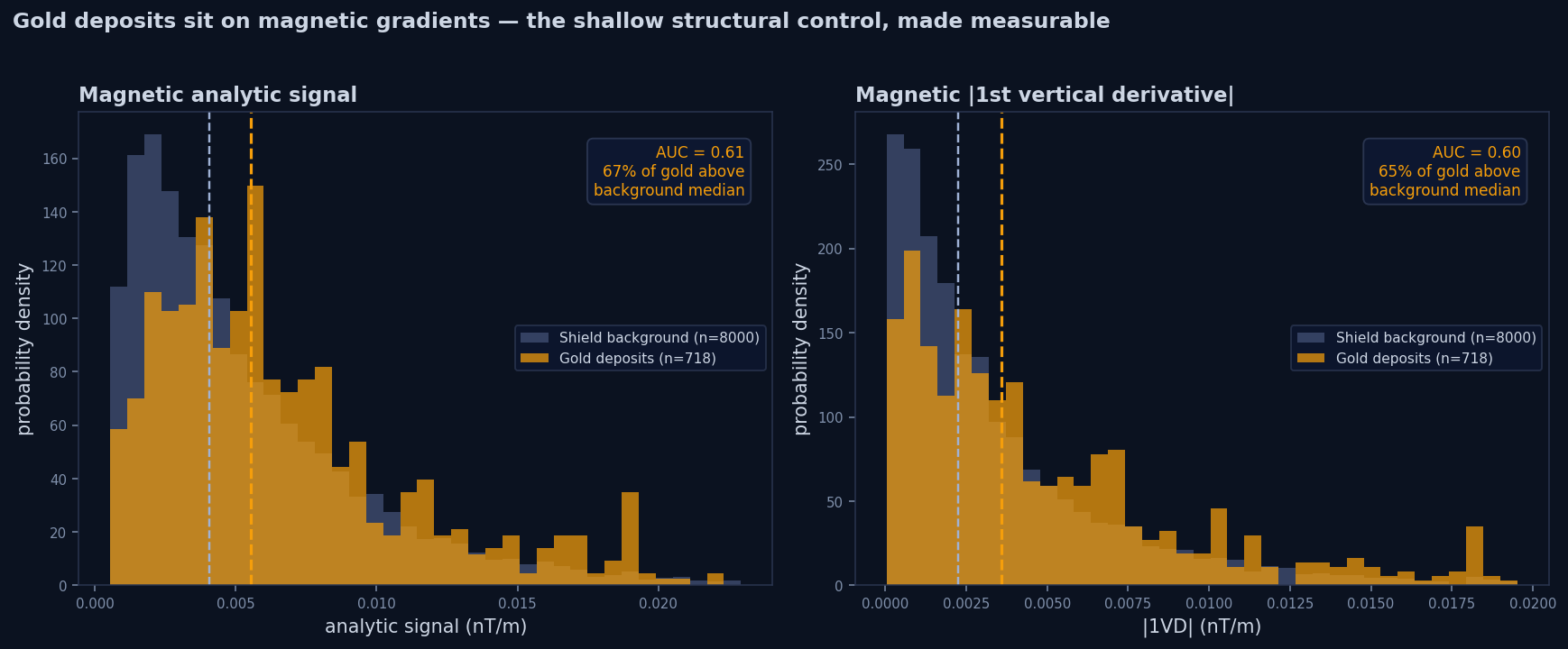
Figure 11.1 — Distribution of the magnetic analytic signal and |1VD| at gold-deposit sites (orange) vs shield background (blue). About two-thirds of deposits exceed the background median. The association is real in this dataset and far stronger than for the raw field — but read it as a promising, testable feature, not a proven control.
That separation is a good start — on raw magnetic amplitude, deposits and background overlap almost completely; after preprocessing, the gradient layers pull them apart. But the same cautions from §9 apply to the magnetics too: the gold points cluster into ~15 belts, so the effective sample is tens, not 718, and the analytic signal is also elevated over basement-versus-cover generally. The filters didn't invent the separation, and they didn't prove a control either — they produced a candidate feature whose predictiveness must be earned through spatially-blocked cross-validation, not declared from a histogram.
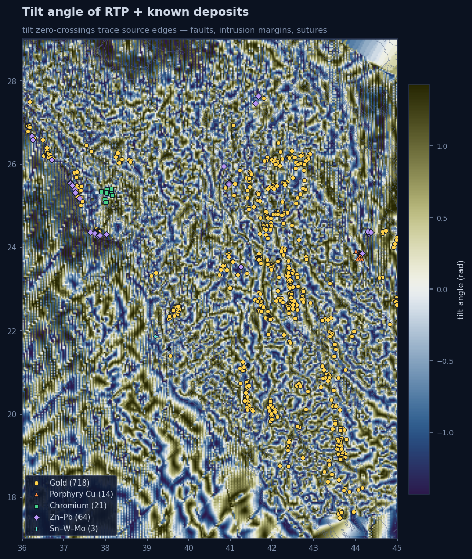
Figure 11.2 — Map view: deposits strung along the tilt-angle discontinuities. The named mineralised corridors (the Nabitah suture, the Wadi Bidah VMS belt and the Wadi Tathlith gold belt) follow magnetic edges that are often interpreted as crustal sutures and shear corridors — a plausible association to test, not a settled one.
Best Practice & Pitfalls
FFT-based filters are exact in theory and fragile in practice. The difference between a feature stack that helps and one that injects artefacts comes down to a few disciplines.
Don't over-interpret — correlation is not control
The biggest trap is not a bad filter; it is a good-looking correlation. Before claiming a layer "predicts" deposits, rule out the obvious: spatial clustering (deposits in belts are pseudo-replicates — decluster, and validate with spatially-blocked folds, never random ones), confounders (here, Bouguer ≈ −0.94 with elevation, so an apparent density signal was mostly topography), and sampling bias (basement-vs-cover, AOI extent). A feature being associated with known deposits earns it a place as a candidate; only honest validation earns it the word "predictive".
Fill gaps before the FFT
The Fourier transform cannot accept missing values — a single NaN poisons the whole grid. Infill data gaps (and re-mask them afterwards if you want honest coverage) before any filter. Global compilations like EMAG2 have real holes; ignore them and every output is empty.
Detrend and pad
Remove a low-order trend and taper/pad the grid edges, or the periodic FFT will wrap the field around and stamp a false high-gradient frame around your area of interest — which a model will happily mistake for structure.
Project to metres, correctly
Derivatives and continuation are defined in metres, not degrees. Reproject to an equal-area or conformal grid before filtering. A naive single-UTM-zone shortcut can mis-register a continental grid by tens of kilometres — moving every feature off its geology.
Get the RTP angles right; respect low latitudes
Use the IGRF inclination/declination for the survey's location and epoch. Below |I| ≈ 15°, switch to reduction-to-equator or the analytic signal, which is direction-independent.
Match resolution to the question
A 3.7 km global grid resolves belts, not drill targets. Use it for regional permissivity; bring in airborne surveys for prospect-scale features. Don't over-claim what a coarse layer can predict.
Takeaway
Geophysical preprocessing is not a beautification step that happens before the "real" modelling. It is the modelling's foundation — the point at which raw physics becomes learnable structure.
The one-paragraph version
Gravity and magnetics carry the crust's structure across continents, but the raw fields disguise it: anomalies are offset, scales are mixed, and amplitude hides faint faults. A small suite of exact, physics-based filters — reduction-to-pole, derivatives, tilt, analytic signal, upward continuation — re-expresses the field as sharp, depth-aware, structure-revealing layers, and that is their real job: turning physics into candidate features. On the Arabian Shield, known gold deposits are measurably enriched on the magnetic gradients those filters reveal, and gravity adds deep-crustal context. We are careful not to call any of it a proven control — apparent associations can be clustering or topography in disguise — but as features, honestly built and honestly validated, they are exactly what an AI needs to read the geology the eye cannot.
Where the features go next
Tutorial 2 takes a stack just like this one and builds the spatial–temporal AI that ranks drill targets.
References
Primary and authoritative sources for the methods, datasets and geology above. Every entry was checked against a resolving DOI or the issuing agency; links go to the publisher of record.
Show full reference list
Potential-field theory & filters
- Baranov, V. (1957). A new method for interpretation of aeromagnetic maps: pseudo-gravimetric anomalies. Geophysics, 22(2), 359–382. doi:10.1190/1.1438369
- Baranov, V., & Naudy, H. (1964). Numerical calculation of the formula of reduction to the magnetic pole. Geophysics, 29(1), 67–79. doi:10.1190/1.1439334
- Blakely, R. J. (1995). Potential Theory in Gravity and Magnetic Applications. Cambridge University Press. doi:10.1017/CBO9780511549816
- Gunn, P. J. (1975). Linear transformations of gravity and magnetic fields. Geophysical Prospecting, 23(2), 300–312. doi:10.1111/j.1365-2478.1975.tb01530.x
- Henderson, R. G., & Zietz, I. (1949). The computation of second vertical derivatives of geomagnetic fields. Geophysics, 14(4), 508–516. doi:10.1190/1.1437558
- Jacobsen, B. H. (1987). A case for upward continuation as a standard separation filter for potential-field maps. Geophysics, 52(8), 1138–1148. doi:10.1190/1.1442378
- Cordell, L. (1979). Gravimetric expression of graben faulting in Santa Fe country and the Española Basin, New Mexico. New Mexico Geological Society Guidebook, 30, 59–64. doi:10.56577/FFC-30.59
- Cordell, L., & Grauch, V. J. S. (1985). Mapping basement magnetization zones from aeromagnetic data in the San Juan basin, New Mexico. In W. J. Hinze (Ed.), The Utility of Regional Gravity and Magnetic Anomaly Maps (pp. 181–197). SEG. doi:10.1190/1.0931830346.ch16
- Blakely, R. J., & Simpson, R. W. (1986). Approximating edges of source bodies from magnetic or gravity anomalies. Geophysics, 51(7), 1494–1498. doi:10.1190/1.1442197
- Nabighian, M. N. (1972). The analytic signal of two-dimensional magnetic bodies with polygonal cross-section: its properties and use for automated anomaly interpretation. Geophysics, 37(3), 507–517. doi:10.1190/1.1440276
- Nabighian, M. N. (1984). Toward a three-dimensional automatic interpretation of potential field data via generalized Hilbert transforms: fundamental relations. Geophysics, 49(6), 780–786. doi:10.1190/1.1441706
- Roest, W. R., Verhoef, J., & Pilkington, M. (1992). Magnetic interpretation using the 3-D analytic signal. Geophysics, 57(1), 116–125. doi:10.1190/1.1443174
- Li, X. (2006). Understanding 3D analytic signal amplitude. Geophysics, 71(2), L13–L16. doi:10.1190/1.2184367
- Miller, H. G., & Singh, V. (1994). Potential field tilt—a new concept for location of potential field sources. Journal of Applied Geophysics, 32(2–3), 213–217. doi:10.1016/0926-9851(94)90022-1
- Verduzco, B., Fairhead, J. D., Green, C. M., & MacKenzie, C. (2004). New insights into magnetic derivatives for structural mapping. The Leading Edge, 23(2), 116–119. doi:10.1190/1.1651454
- Salem, A., Williams, S., Fairhead, J. D., Ravat, D., & Smith, R. (2007). Tilt-depth method: a simple depth estimation method using first-order magnetic derivatives. The Leading Edge, 26(12), 1502–1505. doi:10.1190/1.2821934
- Mendonça, C. A., & Silva, J. B. C. (1993). A stable truncated series approximation of the reduction-to-the-pole operator. Geophysics, 58(8), 1084–1090. doi:10.1190/1.1443492
- Li, X. (2008). Magnetic reduction-to-the-pole at low latitudes: observations and considerations. The Leading Edge, 27(8), 990–1002. doi:10.1190/1.2967550
- Clark, D. A., & Emerson, D. W. (1991). Notes on rock magnetization characteristics in applied geophysical studies. Exploration Geophysics, 22(3), 547–555. doi:10.1071/EG991547
Gravity & geodesy
- Hinze, W. J., von Frese, R. R. B., & Saad, A. H. (2013). Gravity and Magnetic Exploration: Principles, Practices, and Applications. Cambridge University Press. ISBN 978-0-521-87101-3.
- Hackney, R. I., & Featherstone, W. E. (2003). Geodetic versus geophysical perspectives of the "gravity anomaly". Geophysical Journal International, 154(1), 35–43. doi:10.1046/j.1365-246X.2003.01941.x
- Hinze, W. J., et al. (2005). New standards for reducing gravity data: the North American gravity database. Geophysics, 70(4), J25–J32. doi:10.1190/1.1988183
- Li, X., & Götze, H.-J. (2001). Ellipsoid, geoid, gravity, geodesy, and geophysics. Geophysics, 66(6), 1660–1668. doi:10.1190/1.1487109
- Simpson, R. W., Jachens, R. C., Blakely, R. J., & Saltus, R. W. (1986). A new isostatic residual gravity map of the conterminous United States. Journal of Geophysical Research, 91(B8), 8348–8372. doi:10.1029/JB091iB08p08348
Datasets & software
- Maus, S., et al. (2009). EMAG2: a 2-arc min resolution Earth Magnetic Anomaly Grid compiled from satellite, airborne, and marine magnetic measurements. Geochemistry, Geophysics, Geosystems, 10(8), Q08005. doi:10.1029/2009GC002471
- Meyer, B., Saltus, R., & Chulliat, A. (2017). Derivation and error analysis of the Earth Magnetic Anomaly Grid at 2 arc min resolution version 3 (EMAG2v3). Geochemistry, Geophysics, Geosystems, 18(12), 4522–4537. doi:10.1002/2017GC007280 · Data: NOAA NCEI, doi:10.7289/V5H70CVX
- Balmino, G., Vales, N., Bonvalot, S., & Briais, A. (2012). Spherical harmonic modelling to ultra-high degree of Bouguer and isostatic anomalies. Journal of Geodesy, 86(7), 499–520. doi:10.1007/s00190-011-0533-4
- Bonvalot, S., et al. (2012). World Gravity Map (WGM2012). BGI/CGMW/CNES/IRD. doi:10.18168/bgi.23
- Alken, P., et al. (2021). International Geomagnetic Reference Field: the thirteenth generation. Earth, Planets and Space, 73, 49. doi:10.1186/s40623-020-01288-x
- IAGA Working Group V-MOD (2024). International Geomagnetic Reference Field, 14th generation (IGRF-14) [Data set]. Zenodo. doi:10.5281/zenodo.14012303
- Uieda, L., & the Fatiando a Terra developers (2024). Harmonica: forward modeling, inversion, and processing gravity and magnetic data [Software]. Zenodo. doi:10.5281/zenodo.3628741
- Abdelrahman, K., et al. (2024). Structural mapping of the west central Arabian Shield (Saudi Arabia) using downward continued magnetic data. Journal of King Saud University – Science, 36(2), 103039. doi:10.1016/j.jksus.2023.103039
Arabian Shield geology & deposits
- Stern, R. J. (1994). Arc assembly and continental collision in the Neoproterozoic East African Orogen. Annual Review of Earth and Planetary Sciences, 22, 319–351. doi:10.1146/annurev.ea.22.050194.001535
- Johnson, P. R., et al. (2011). Late Cryogenian–Ediacaran history of the Arabian–Nubian Shield. Journal of African Earth Sciences, 61(3), 167–232. doi:10.1016/j.jafrearsci.2011.07.003
- Stern, R. J., Johnson, P. R., Kröner, A., & Yibas, B. (2004). Neoproterozoic ophiolites of the Arabian–Nubian Shield. In T. M. Kusky (Ed.), Precambrian Ophiolites and Related Rocks (Developments in Precambrian Geology 13, pp. 95–128). Elsevier. doi:10.1016/S0166-2635(04)13003-X
- Johnson, P. R., Abdelsalam, M. G., & Stern, R. J. (2003). The Bi'r Umq–Nakasib suture zone in the Arabian–Nubian Shield. Gondwana Research, 6(3), 523–530. doi:10.1016/S1342-937X(05)71003-0
- Stoeser, D. B., & Camp, V. E. (1985). Pan-African microplate accretion of the Arabian Shield. GSA Bulletin, 96(7), 817–826. doi:10.1130/0016-7606(1985)96<817:PMAOTA>2.0.CO;2
- Worl, R. G. (1979). The Jabal Ishmas–Wadi Tathlith gold belt, Kingdom of Saudi Arabia (USGS Open-File Report 79-1519). doi:10.3133/ofr791519
- Volesky, J. C., Stern, R. J., & Johnson, P. R. (2003). Geological control of massive sulfide mineralization in the Neoproterozoic Wadi Bidah shear zone, southwestern Saudi Arabia. Precambrian Research, 123(2–4), 235–247. doi:10.1016/S0301-9268(03)00070-6
- Abu-Alam, T. S., Abd El Monsef, M., & Grosch, E. (2019). Shear-zone hosted gold mineralization of the Arabian–Nubian Shield. Geological Society, London, Special Publications, 478, 287–307. doi:10.1144/SP478.13
Machine learning & statistical methodology
- Bonham-Carter, G. F. (1994). Geographic Information Systems for Geoscientists: Modelling with GIS. Pergamon. ISBN 0-08-041867-8.
- Carranza, E. J. M. (2008). Geochemical Anomaly and Mineral Prospectivity Mapping in GIS. Elsevier. ISBN 978-0-444-51325-0.
- Rodriguez-Galiano, V., et al. (2015). Machine learning predictive models for mineral prospectivity: an evaluation of neural networks, random forest, regression trees and support vector machines. Ore Geology Reviews, 71, 804–818. doi:10.1016/j.oregeorev.2015.01.001
- Zuo, R. (2020). Geodata science-based mineral prospectivity mapping: a review. Natural Resources Research, 29(6), 3415–3424. doi:10.1007/s11053-020-09700-9
- Domingos, P. (2012). A few useful things to know about machine learning. Communications of the ACM, 55(10), 78–87. doi:10.1145/2347736.2347755
- Roberts, D. R., et al. (2017). Cross-validation strategies for data with temporal, spatial, hierarchical, or phylogenetic structure. Ecography, 40(8), 913–929. doi:10.1111/ecog.02881
- Ploton, P., et al. (2020). Spatial validation reveals poor predictive performance of large-scale ecological mapping models. Nature Communications, 11, 4540. doi:10.1038/s41467-020-18321-y
- Meyer, H., & Pebesma, E. (2022). Machine learning-based global maps of ecological variables and the challenge of assessing them. Nature Communications, 13, 2208. doi:10.1038/s41467-022-29838-9
- Hurlbert, S. H. (1984). Pseudoreplication and the design of ecological field experiments. Ecological Monographs, 54(2), 187–211. doi:10.2307/1942661
- Hanley, J. A., & McNeil, B. J. (1982). The meaning and use of the area under a receiver operating characteristic (ROC) curve. Radiology, 143(1), 29–36. doi:10.1148/radiology.143.1.7063747
- Hosmer, D. W., Lemeshow, S., & Sturdivant, R. X. (2013). Applied Logistic Regression (3rd ed.). Wiley. doi:10.1002/9781118548387