Big picture → Intuition → Physics → Data → Methods → Results → AI
Geological Mapping from Space: From Spectral Physics to AI-Powered Lithology
Rocks speak in light. Every mineral absorbs and reflects electromagnetic radiation at wavelengths governed by its chemistry and crystal structure. Satellite sensors record this spectral language, and geologists decode it into geological maps. This tutorial teaches you the full chain — from the physics of mineral absorption, through traditional remote sensing workflows, all the way to modern machine learning — using real data from the Nidar Ophiolite Complex in the Trans-Himalayan terrain of Ladakh.
Continue to Tutorial 2: AI-Driven Mineral Prospectivity →By the end of this tutorial you will be able to:
- Explain how mineral chemistry controls spectral reflectance from visible to thermal infrared wavelengths.
- Select the right satellite sensor based on your geological objective and the spectral/spatial constraints of each mission.
- Execute a full preprocessing pipeline from at-sensor radiance to atmospherically corrected surface reflectance.
- Apply and interpret FCC, PCA, band indices, and supervised classifiers (Minimum Distance, Maximum Likelihood, SAM).
- Understand what makes hyperspectral data qualitatively different from multispectral data for mineral mapping.
- Design an AI/ML geological mapping workflow grounded in physical features and geological validation.
- Integrate multi-sensor evidence to confidently discriminate dunite, peridotite, gabbro, and serpentinization in a real ophiolite setting.
Why Satellite Mapping for Geology?
Before we talk about wavelengths or algorithms, we need to answer a more fundamental question: why are we doing this at all? Traditional geological mapping is painstaking, expensive, and physically dangerous in high-altitude terrains. Satellite remote sensing does not replace the geologist in the field — but it extends their reach dramatically.
The Problem: Terrain That Cannot Be Mapped on Foot
The Nidar Ophiolite Complex sits in the Trans-Himalayan belt of Ladakh at elevations exceeding 4,000 m. Access is seasonal, roads are unreliable, and the terrain is steep and glaciated. A single field campaign can cover at most a few transects across a region spanning hundreds of square kilometres. Important lithological contacts — the boundary between a dunite body and serpentinized peridotite, for instance — can sit on a cliff face that no geologist will ever stand on.
This is the fundamental problem that satellite remote sensing solves. A satellite passes over the same area every few days, collects spectral data wall-to-wall, and delivers that data for processing from a desktop. Regional geological patterns become visible in hours rather than seasons.
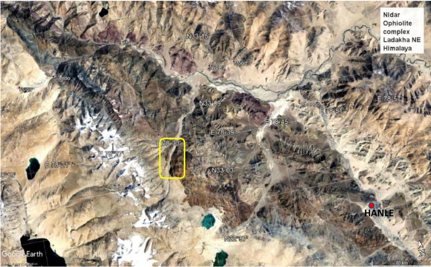
Figure 1.1 — Satellite view of the Nidar Ophiolite Complex (Google Earth). High-altitude, structurally complex terrain like this is mapped continuously and synoptically from orbit, while ground traverses cover only narrow accessible corridors. Source: Ghaste (2020).
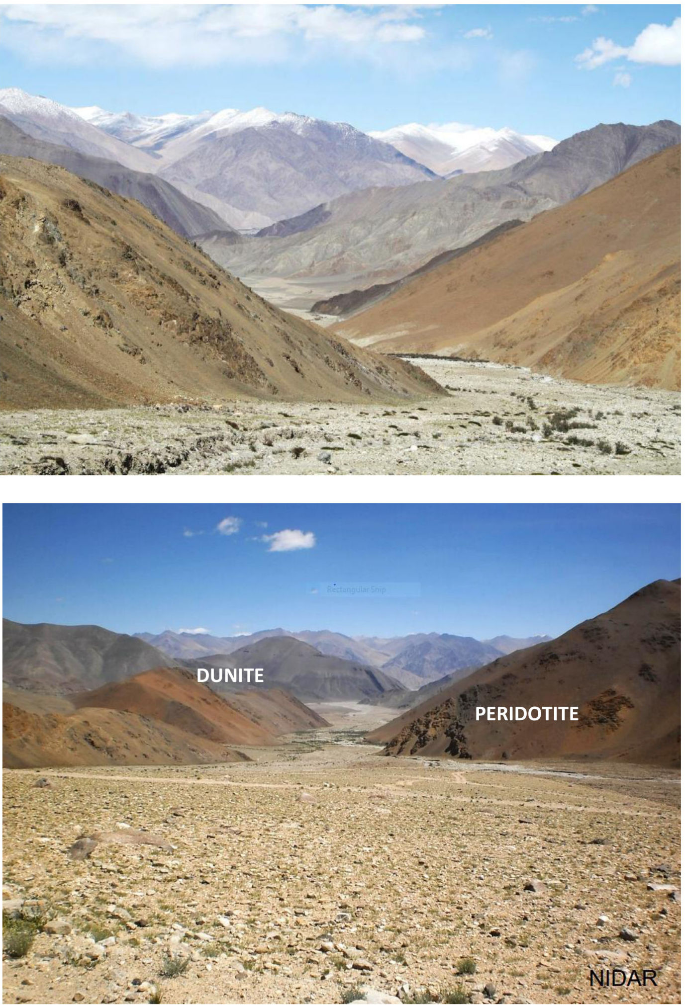
Figure 1.2 — Dunite outcrops along the Nidar Valley. The valley exposes the ultramafic mantle sequence (dunite, peridotite) and overlying mafic units in vertical succession — geologically ideal for remote-sensing validation but logistically challenging to traverse comprehensively on foot. Source: Ghaste (2020).
Traditional Mapping vs Satellite-Assisted Mapping
| Aspect | Field-Only Mapping | Satellite-Assisted Mapping |
|---|---|---|
| Spatial coverage | Narrow transects; patchy in inaccessible terrain | Continuous wall-to-wall; 100% scene coverage |
| Confidence at sample sites | Very high (hand specimen, thin section) | High where calibrated; lower in shadows/mixed pixels |
| Regional lithological context | Inferred from transects; can miss major units | Directly observable at regional scale |
| Temporal repeatability | One campaign per season | Multi-temporal; seasonal changes trackable |
| Cost per km² | Very high in remote terrain | Low (imagery often open-access) |
| Detection of alteration fronts | Only at exposure; requires luck | Detectable via spectral indices over large areas |
Key Insight
Satellite mapping is strongest when used as a hypothesis engine: it detects regional spectral patterns, highlights candidate lithological contacts, and tells you exactly where to go in the field. The field campaign then validates, refines, and adds petrographic ground truth that satellites cannot provide. Neither approach alone is sufficient for a rigorous geological map.
The Decision Framework
Before starting any satellite-based geological mapping project, ask these three questions:
Regional lithology mapping requires different sensors and methods than detection of a specific alteration mineral. Define your target (lithological unit, mineral, alteration zone) before choosing a dataset.
If dunite bodies are 10–100 m wide and your pixel is 30 m, you will lose a significant proportion of them in mixed pixels. Match pixel size to expected unit size.
Published field maps, existing sample collections, and thin section records all constrain where you place training ROIs and how you interpret classification outputs.
Common Mistake
Treating a classified satellite map as geological ground truth. A classification product is a spectral interpretation. It must be cross-checked against field observations, published geology, and petrographic descriptions before being accepted as a geological map.
Understanding Spectral Signatures
Before you can interpret a satellite image geologically, you need to understand why rocks look different at different wavelengths. This is not intuitive — two rocks that look identical in a photograph can be completely different spectrally in the shortwave infrared. The physics behind this is where geological remote sensing begins.
The Physics of Spectral Reflectance
When sunlight hits a rock surface, three things can happen to the incoming photons: they can be reflected (bounced back toward the sensor), absorbed (their energy taken up by the material), or transmitted (passed through, rare in opaque rocks). The reflectance at any given wavelength is simply the fraction of incoming energy that is reflected.
A reflectance spectrum plots this fraction against wavelength across the electromagnetic spectrum — from visible light (~400–700 nm) through near-infrared (NIR, ~700–1000 nm), shortwave infrared (SWIR, ~1000–2500 nm), and thermal infrared (TIR, ~8,000–12,000 nm). Geologically, the most diagnostic information lives in the SWIR, where molecular bonds in minerals produce characteristic absorption features.
Figure 2.1 — Conceptual reflectance spectra for peridotite, dunite, and gabbro across the VIS–SWIR range. Spectral absorption troughs are the key to discrimination. Note: wavelength axis is compressed for TIR for display clarity.
The Three Key Absorption Mechanisms
Iron Electronic Transitions (VIS–NIR)
Iron is the workhorse of geological remote sensing. In its ferrous (Fe²⁺) state, iron in silicate minerals like olivine and pyroxene creates broad absorption features around 900–1100 nm. The exact position depends on the mineral host: olivine absorbs near 860 nm and 1050 nm, while clinopyroxene absorbs near 1000–1100 nm.
Ferric iron (Fe³⁺) — the oxidized form, common in weathered or hydrothermally altered rocks — produces absorptions around 400–900 nm, giving iron-rich surfaces their characteristic orange-brown colour. The Fe²⁺/Fe³⁺ ratio is a proxy for alteration state.
Hydroxyl & Water Molecular Vibrations (SWIR)
The shortwave infrared (1000–2500 nm) is dominated by molecular vibrations. The OH (hydroxyl) group and H₂O (water) both absorb strongly around ~1400 nm and ~1900 nm due to overtone and combination vibrations. These are diagnostic of hydrated minerals and serpentinization.
In serpentinized peridotites, hydrothermal water replaces olivine with serpentine minerals (antigorite, chrysotile, lizardite), dramatically changing the SWIR spectrum and making serpentinization detectable from orbit.
Mg-OH Vibrations (~2200–2350 nm)
This is the most geologically diagnostic feature for ultramafic rocks. The Mg-OH bond produces a combination absorption near ~2300 nm. In serpentine-group minerals — which form when olivine-rich peridotite or dunite is hydrated — this feature is particularly strong.
From the Nidar study: absorption near 2300 nm in peridotite specimens (e.g., sample Pd-1) can be attributed to Mg-OH in serpentine, while a small absorption near 2130 nm is due to a different Mg-OH configuration, giving an M-shape to the spectrum between 2077–2166 nm. Gabbro, with its pyroxene content, shows a contrasting W-shape feature at 2200–2400 nm.
Rock-Specific Spectral Fingerprints (from Nidar field samples)
The following table summarises the key absorption positions measured from field-collected specimens in the Nidar study and their physical causes. These spectral fingerprints are what classifiers use to separate rock types.
| Rock Type | Key Absorption Positions (nm) | Physical Cause |
|---|---|---|
| Peridotite | 960, 1400, 1740, 1860, 1900, 2100, 2300, 2340, 2420 | Fe²⁺ in olivine+orthopyroxene (960 nm); OH/H₂O from serpentinization (1400, 1900); Mg-OH in serpentine (2100, 2300) |
| Dunite | 860, 1050, 2250 (diagnostic dip) | Fe²⁺ in olivine; SWIR dip at 2250 nm from serpentine group (weathering product) |
| Gabbro | ~1000–1100 (Cpx), 2200–2400 (W-shape) | Fe²⁺ in clinopyroxene (1000–1100); pyroxene feature creates W-shaped double trough at 2200–2400 |
| Chromite | Flat, dark, featureless | Spinel-group opaque mineral; very low overall reflectance with no diagnostic absorption features |
| Pillow Basalt | ~900 nm broad | Fe²⁺ in glassy groundmass |
| Serpentinite | 1400, 1900, 2100, 2300 (strong), 2350 | Fe+Mg-OH overtones in serpentine minerals (antigorite, chrysotile, lizardite) |
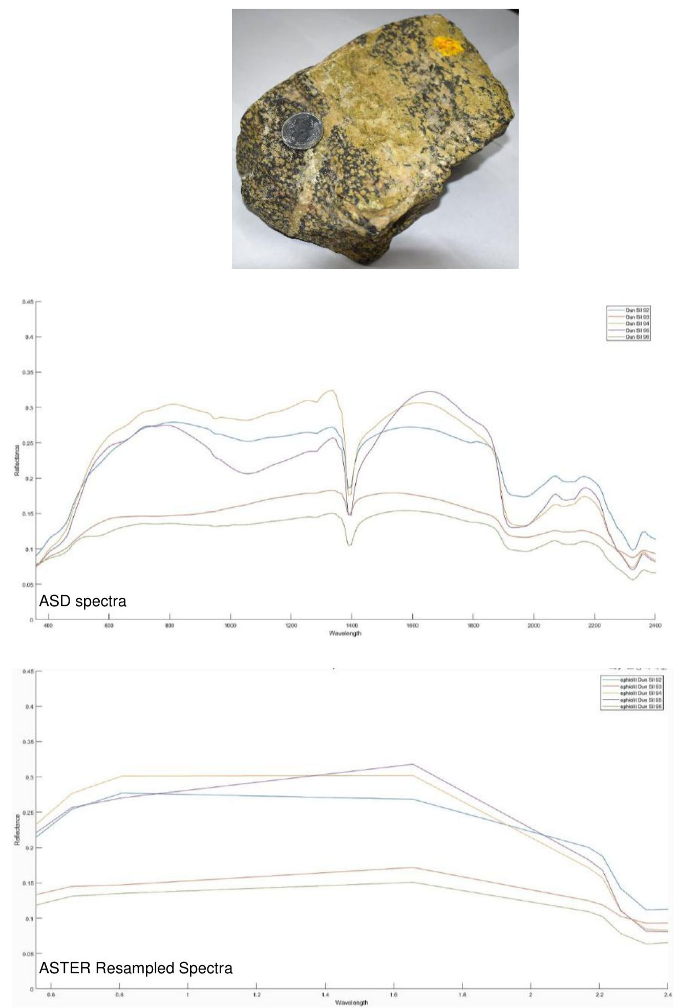
Figure 2.2a — ASD field-measured spectra (top) and ASTER-resampled spectra (bottom) for dunite sample Dun-1. The diagnostic Mg-OH absorption near 2250 nm — caused by serpentinization of olivine — is preserved when the high-resolution field spectrum is resampled to ASTER's 9 SWIR bands. Source: Ghaste (2020).
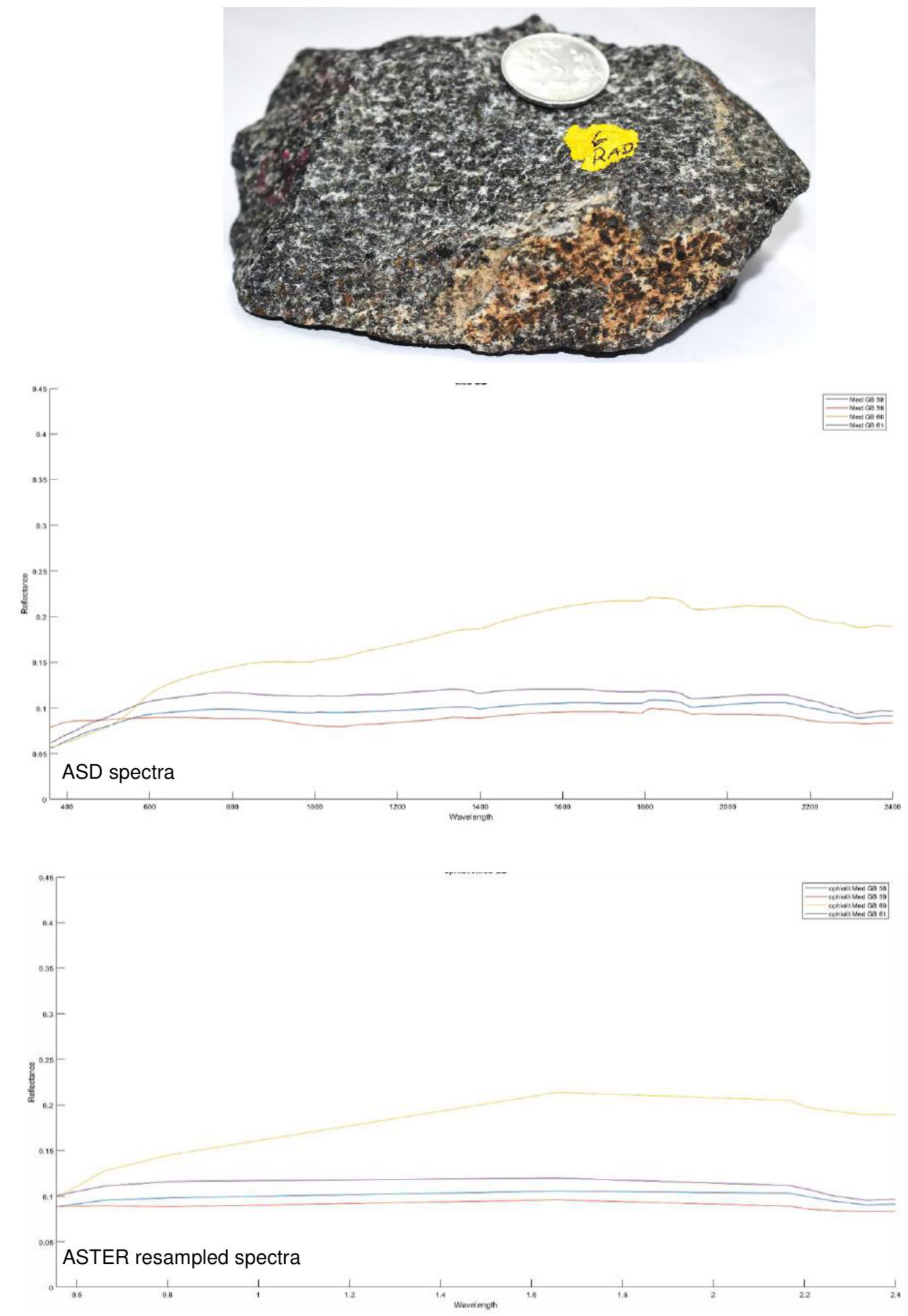
Figure 2.2b — ASD and ASTER-resampled spectra for gabbro (sample Gb-1). The characteristic W-shape double-trough between 2150–2350 nm is caused by pyroxene Fe absorption — a fundamentally different spectral fingerprint from dunite (Fig. 2.2a) that enables unambiguous lithological discrimination from satellite data. Source: Ghaste (2020).
How to Read a Spectrum: A Step-by-Step Sequence
Is the spectrum bright (high albedo) or dark? A high overall reflectance suggests quartz or feldspar-rich lithology. Very dark spectra across all wavelengths suggest mafic oxides like chromite or magnetite.
A rising slope from VIS to NIR suggests dominantly ferrous minerals. A flat or falling slope may indicate more oxidised (Fe³⁺-dominated) or felsic material.
This is the geologically richest region. Mark any troughs between 1000–2500 nm. Ask: is there a feature at ~1400/1900 nm (OH/H₂O)? At ~2100–2300 nm (Mg-OH, serpentine)? At ~2350 nm (Mg-OH + carbonate)? What is the exact shape — a single V or a double W?
A deep, sharp absorption indicates high mineral abundance and purity. A shallow, asymmetric feature may indicate mixing with other minerals or partial serpentinization.
Match your observed spectrum against the USGS Spectral Library or your field-measured ASD spectra. Look for shape correspondence, not just position, because spectral mixing and weathering shift positions slightly.
Analogy: Rocks as musical instruments
Think of the electromagnetic spectrum as a piano keyboard stretching from ultraviolet through thermal infrared. Every wavelength is a key. When light strikes a rock, the minerals inside selectively "press down" certain keys — absorbing energy at those wavelengths. The sensor records which keys are loud (high reflectance) and which are muted (absorption troughs). A reflectance spectrum is the rock's unique chord. Just as a trained musician can identify an instrument by its overtone structure, a spectroscopist can identify a mineral assemblage by its pattern of absorption features.
Key Insight
Lithological discrimination is almost never about a single wavelength. It is about the pattern of features across many wavelengths simultaneously. This is why classifiers that use spectral shape (like SAM) outperform those that use only brightness (like simple thresholding), and why more spectral bands — all else being equal — improve discrimination.
Satellite Datasets Explained
Not all satellites see geology the same way. The choice of sensor directly controls which spectral features you can detect, how large a geological unit must be to appear in a pixel, and how much preprocessing is required. This section introduces the three sensors used in the Nidar study and teaches you to select the right tool for each geological objective.
Sentinel-2: High Resolution Context Mapping
Sentinel-2 is part of ESA's Copernicus programme and provides the highest spatial resolution of the three sensors used in this study. It carries the MultiSpectral Instrument (MSI) with 13 spectral bands. For geology, the most useful are the four 10 m VNIR bands (Blue, Green, Red, NIR) and the 20 m SWIR bands (Band 11 at 1610 nm and Band 12 at 2190 nm).
The limitation for geological work is critical: Sentinel-2 has only two SWIR bands, separated by a wide spectral gap. This means it cannot resolve the detailed absorption shapes that distinguish dunite from peridotite or detect the Mg-OH feature at 2300 nm with confidence. What Sentinel-2 is excellent for is providing spatial context — a high-resolution base map for tracing structural features and broad lithological units, particularly the contrast between mafic/ultramafic rocks and surrounding sedimentary sequences.
In the Nidar study, the Sentinel-2 FCC (Band 11 Red, Band 12 Green, Band 8A Blue) clearly distinguished mafic–ultramafic rocks (pinkish-brown tones) from the sedimentary suite (yellowish-green tones). However, within the ophiolite itself, Gabbro, Peridotite, and Indus Formation could not be separated because their spectral trends are too similar in the limited SWIR bands. Only Dunite, with its characteristic dip at ~2250 nm falling within Band 12, showed a distinctive signature.
Sentinel-2 Specifications (Geology-relevant bands)
| Band | Name | Central Wavelength (nm) | Resolution (m) |
|---|---|---|---|
| B2 | Blue | 490 | 10 |
| B3 | Green | 560 | 10 |
| B4 | Red | 665 | 10 |
| B8 | NIR (broad) | 842 | 10 |
| B8A | NIR (narrow) | 865 | 20 |
| B11 | SWIR-1 | 1610 | 20 |
| B12 | SWIR-2 | 2190 | 20 |
ASTER: The Workhorse of Geological Mapping
ASTER (Advanced Spaceborne Thermal Emission and Reflection Radiometer) is the most powerful of the three sensors for geological mapping. It provides 14 spectral bands spanning VNIR (4 bands at 15 m), SWIR (6 bands at 30 m), and TIR (5 bands at 90 m). This combination is uniquely suited to ophiolite mapping because the SWIR bands capture mineral absorption features between 1.6–2.43 μm — exactly where serpentine, pyroxene, and carbonate produce diagnostic signals — and the TIR bands capture spectral emissivity variations tied to bulk silica content and mineral structure.
The key insight about ASTER's TIR capability: ultramafic rocks (peridotite, dunite) have high silica deficiency relative to mafic rocks (gabbro), and this difference is encoded in emissivity. Ultramafic rocks show higher emissivity at ASTER bands 10–12 and lower emissivity at bands 13–14, while gabbro shows the reverse pattern. This makes thermal emissivity a complementary and independent diagnostic tool.
ASTER Specifications (all 14 bands)
| Region | Band | Wavelength (μm) | Resolution (m) |
|---|---|---|---|
| VNIR | 1 | 0.52–0.60 (Green) | 15 |
| 2 | 0.63–0.69 (Red) | 15 | |
| 3N | 0.78–0.86 (NIR nadir) | 15 | |
| 3B | 0.78–0.86 (NIR back) | 15 | |
| SWIR | 4 | 1.60–1.70 | 30 |
| 5 | 2.145–2.185 | 30 | |
| 6 | 2.186–2.225 | 30 | |
| 7 | 2.235–2.285 | 30 | |
| 8 | 2.295–2.365 | 30 | |
| 9 | 2.360–2.430 | 30 | |
| TIR | 10 | 8.125–8.475 μm | 90 |
| 11 | 8.475–8.825 μm | 90 | |
| 12 | 8.925–9.275 μm | 90 | |
| 13 | 10.25–10.95 μm | 90 | |
| 14 | 10.95–11.65 μm | 90 |
Hyperion: Continuous Hyperspectral Coverage
Hyperion, aboard NASA's EO-1 satellite, is a hyperspectral imager providing 242 unique spectral channels from 450 nm to 2500 nm at 30 m spatial resolution and 10 nm spectral bandwidth. While Sentinel-2 samples the SWIR at only 2 points and ASTER at 6, Hyperion samples it at over 170 channels — enough to resolve the full shape of every absorption feature.
This spectral density enables a qualitatively different kind of analysis. Rather than detecting that an absorption exists somewhere near 2300 nm, Hyperion lets you resolve the exact shape and position of the Mg-OH feature, discriminating between different serpentine polymorphs (antigorite vs chrysotile vs lizardite) or quantifying the degree of serpentinization. The trade-off is a narrow swath width (7.75 km) and a more demanding preprocessing and noise-removal workflow.
Hyperion Specifications
| Parameter | Value |
|---|---|
| Spectral range | 450–2500 nm (full VIS–SWIR) |
| Spectral sampling interval | 10 nm (nominal) |
| Number of channels | 242 unique (from 220 bands) |
| VNIR channels | 70 (356–1058 nm) |
| SWIR channels | 172 (852–2577 nm) |
| Spatial resolution | 30 m |
| Swath width | 7.75 km |
| Digitization | 12 bits |
Side-by-Side Comparison
| Property | Sentinel-2 | ASTER | Hyperion |
|---|---|---|---|
| Number of geology-useful bands | 7 (VNIR+SWIR) | 14 (VNIR+SWIR+TIR) | ~200+ (VNIR+SWIR) |
| SWIR coverage | 2 bands (1610, 2190 nm) | 6 bands (1.6–2.43 μm) | Continuous 1000–2500 nm |
| Thermal infrared | None | 5 bands (8–12 μm) | None |
| Spatial resolution (geology bands) | 10–20 m | 15–90 m | 30 m |
| Scene coverage | Wide (110×110 km) | Wide (60×60 km) | Narrow (7.75×185 km) |
| Can detect serpentinization? | Partially (2190 nm only) | Yes (5/7 band ratio) | Yes (full feature shape) |
| Separates gabbro from peridotite? | Difficult; limited SWIR | Good (SWIR shape + TIR) | Excellent (full SWIR curve) |
Key Insight: Why Multi-Sensor?
No single sensor does everything. Sentinel-2 provides the spatial precision to trace contacts. ASTER provides the spectral depth for lithological separation and thermal confirmation. Hyperion provides the spectral resolution for confident endmember identification and mineral mapping. The most reliable geological maps combine evidence from all three.
Common Mistake
Using Sentinel-2 alone and reporting that dunite and peridotite "cannot be separated." This is a sensor limitation, not a geological one. ASTER's six SWIR bands — especially the contrast between bands 4 (1.65 μm) and 7 (2.26 μm) — clearly separates these units. Always match the sensor to the question before concluding that separation is impossible.
Preprocessing Pipeline: From Radiance to Reflectance
A raw satellite image does not record the spectral properties of rocks. It records radiance at the sensor — electromagnetic energy that has been reflected from the surface, scattered by the atmosphere, and detected by the sensor. Before any geological analysis, this radiance must be converted into at-surface reflectance. This step is not cosmetic; it is the difference between a spectrum that physically describes your rock and one that describes your atmosphere.
Why the Atmosphere Matters
Sunlight must travel twice through the atmosphere: once on the way down to the surface, and once on the way back up to the satellite. In that journey, atmospheric gases (particularly water vapour, carbon dioxide, and ozone), aerosols, and haze do two things:
- Absorption: Specific wavelength ranges are absorbed almost completely (e.g., ~1400 nm and ~1900 nm are dominated by water vapour absorption — making spectral features at those wavelengths unreliable).
- Scattering: Short wavelengths (blue/UV) are scattered more than long wavelengths (Rayleigh scattering), adding a diffuse glow that inflates reflectance estimates at short wavelengths.
Without correction, a geologist comparing a SWIR spectrum from a satellite image to a laboratory ASD measurement will find a mismatch. The absorption features may be present, but their depth and shape will be systematically distorted by atmospheric effects. Classification based on uncorrected imagery will produce spectral mismatches — and ultimately, misclassified lithology.
Figure 4.1 — End-to-end preprocessing pipeline. FLAASH (Fast Line-of-sight Atmospheric Analysis of Spectral Hypercubes) is the critical correction step, converting at-sensor radiance to true at-surface reflectance using MODTRAN-based radiative transfer modelling.
FLAASH in Depth
FLAASH was applied in the Nidar study for both ASTER and Hyperion. For ASTER, suitable atmospheric parameters are selected via MODTRAN (Moderate Resolution Atmospheric Transmittance and Radiance), a physics-based radiative transfer model. A scaled DISORT MODTRAN multi-scatter model with 8 streams was used — this setting balances computational speed with accuracy for high-altitude arid terrain.
The effect of FLAASH is profound at key wavelengths. In the SWIR, where absorption features are diagnostic of mineral composition, uncorrected imagery may show artificially shallow or shifted troughs. After FLAASH correction, spectral profiles extracted from the image can be directly compared to field-measured ASD spectra and USGS library spectra.
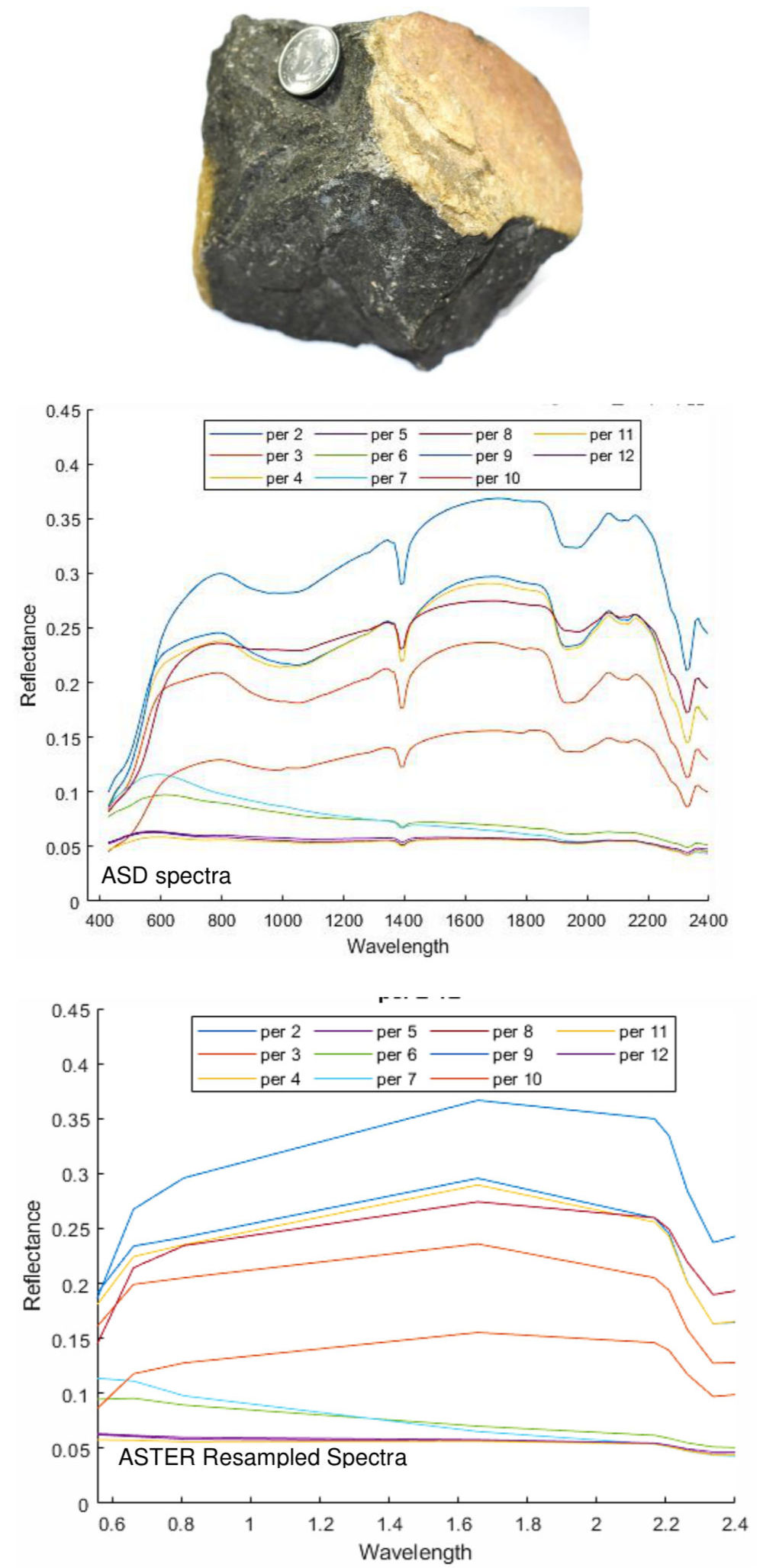
Figure 4.2 — ASD field spectra (top) and ASTER-resampled spectra (bottom) for a peridotite sample. The characteristic Mg-OH absorption near 2300 nm — diagnostic of serpentinization — is clearly visible in both representations. After atmospheric correction, this feature is preserved in the satellite signal; without correction, it is masked by atmospheric water-vapour absorption. Source: Ghaste (2020).
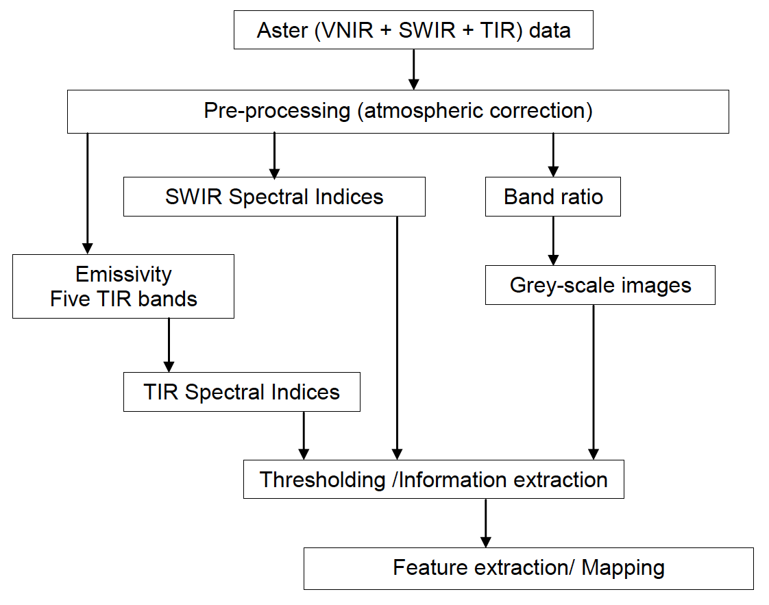
Figure 4.3 — Complete ASTER image-processing workflow for lithological mapping within an ophiolite suite. After atmospheric correction, the SWIR branch (band ratios, spectral indices) and the TIR branch (emissivity, mineral indices) operate in parallel, producing complementary evidence streams that are fused at the final mapping stage. Source: Ghaste (2020), thesis Fig. 8.
Preprocessing Quality Checklist
Common Mistake
Applying atmospheric correction as a single automated step without checking output spectra. In high-altitude terrain with variable aerosol loading (such as Ladakh), incorrect FLAASH parameters can leave residual path radiance in SWIR bands — making ultramafic rocks appear to have weaker Mg-OH features than they truly do, which directly degrades serpentinization detection.
Traditional Mapping Workflow
Once your imagery is atmospherically corrected, you have a stack of physically meaningful reflectance values. Now the geological interpretation begins. The traditional workflow follows a logical sequence: visualise, inspect, compress, index, classify, validate. Each step builds evidence.
A) False Color Composites (FCC)
A False Color Composite assigns different spectral bands to the red, green, and blue display channels. This exploits the human eye's sensitivity to colour to reveal spectral contrasts that are invisible in natural-colour images. In geological remote sensing, FCC is always the first step — before indices, before classification. It tells you whether there is any spectral structure worth analysing further.
Why ASTER 7-4-2 (Red-Green-Blue) for ophiolite mapping?
Each band is selected for a physical reason:
- Band 7 (Red, 2.266 μm) — Sensitive to Mg-OH-rich minerals and carbonates in serpentinized peridotites. Highlights zones with strong Mg-OH absorption.
- Band 4 (Green, 1.656 μm) — Shows high reflectance in dunite. Also highlights hydroxyl-bearing and serpentine minerals in serpentinized harzburgites/peridotites.
- Band 2 (Blue, 0.661 μm) — Highlights weathered iron minerals from olivine/pyroxene-rich peridotites (Fe³⁺ transitions).
The resulting FCC dramatically enhances contrast. In the Nidar study: Dunite appears bright green (high Band 4 reflectance); Peridotite appears dark brown; Gabbro appears light greenish; Lian Molasse appears cream-white; Chert-Jasper sediments appear bright yellow; Tso Morari crystalline appears greenish-yellow; and the contact between crystalline basement and the ophiolite is clearly traceable.
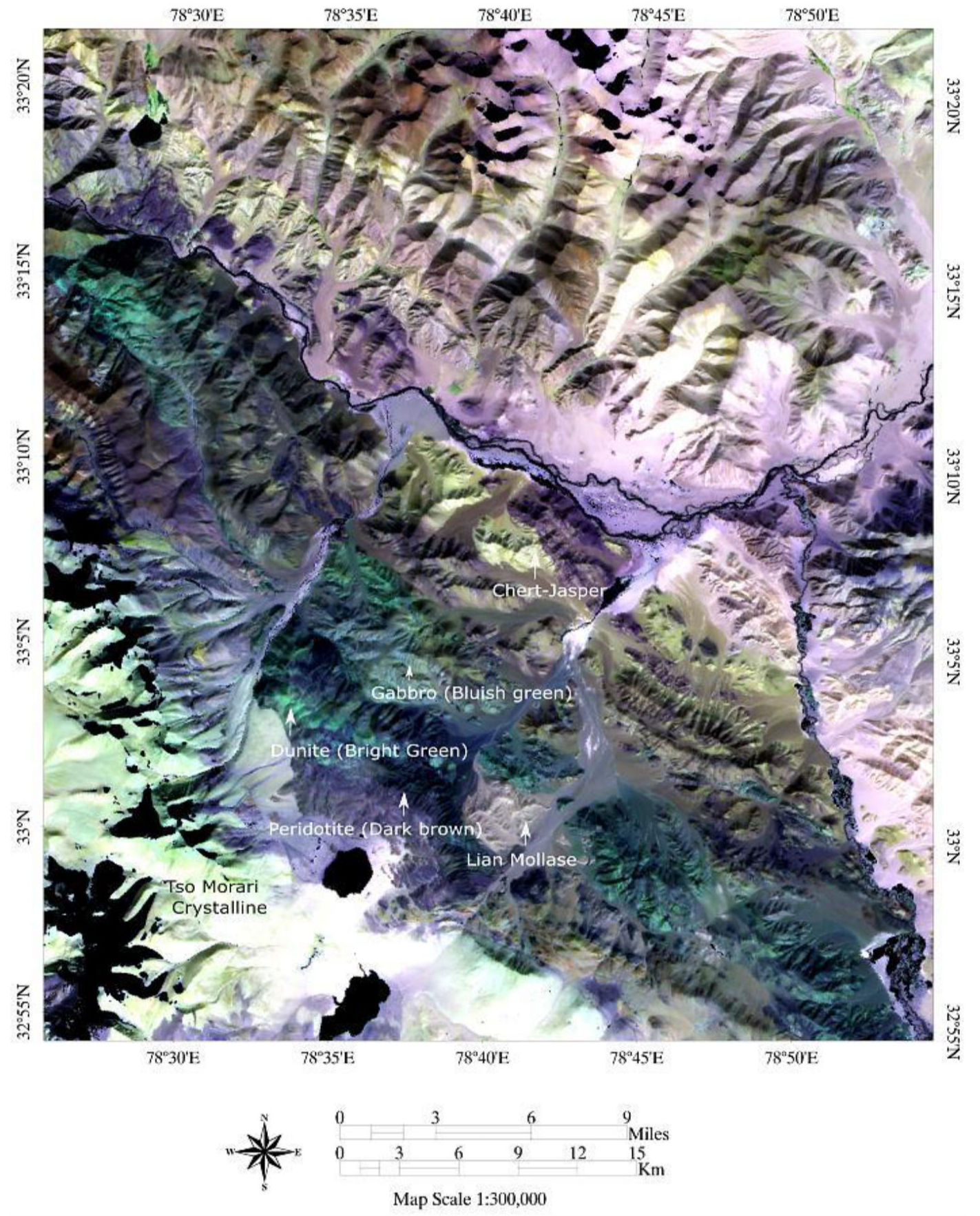
Figure 5.1 — ASTER False-Colour Composite (Band 7 → Red, Band 4 → Green, Band 2 → Blue) showing strong colour contrast between lithological units at the Nidar Ophiolite Complex. Each unit's apparent colour arises directly from differences in mineralogy: dunite appears bright green, peridotite dark brown, gabbro light greenish, the Lian Molasse cream-white, and the Tso Morari crystalline greenish-yellow. Source: Ghaste (2020), thesis Fig. 32.
Key Insight
In a well-designed FCC, each colour corresponds to a physical spectral behaviour. Geological interpretation begins by asking: "What mineral property explains this colour?" not "What colour looks like the rock I expect?" The latter leads to confirmation bias; the former leads to discovery.
B) Spectral Profiles and ROI Analysis
Once the FCC reveals potential lithological zones, you extract spectral profiles from Regions of Interest (ROIs) within those zones. An ROI is a set of pixels that represents a known (or hypothesised) geological unit. The shape of the extracted spectrum is your primary interpretive tool.
The V-shape vs W-shape diagnostic (from Nidar study)
In ASTER SWIR box plots extracted from ROIs at Nidar (Figure 5.2), a crucial diagnostic pattern emerges in the 2150–2400 nm window:
- Peridotite shows a characteristic V-shaped dip — a single broad trough centred near ~2300 nm, consistent with Mg-OH in serpentine minerals replacing olivine.
- Gabbro shows a W-shaped double dip — a reflection peak near 2250 nm (Band 7) flanked by two troughs at ~2200 nm and ~2350 nm, caused by pyroxene absorptions.
- Dunite shows elevated reflectance at Band 4 (1656 nm) compared to peridotite, then a dip at ~2250 nm from serpentine.
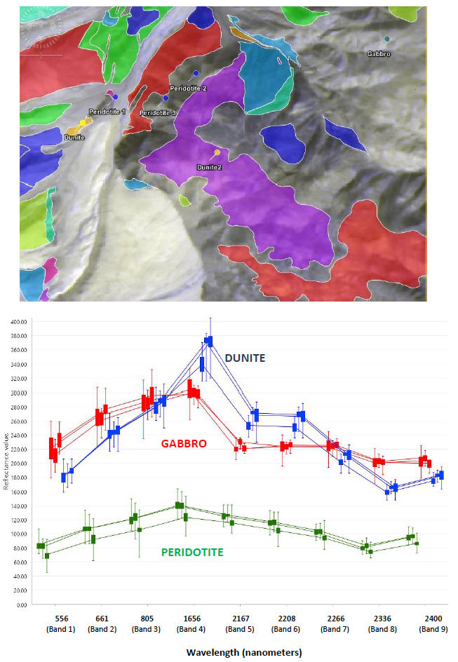
Figure 5.2 — Box plots of ASTER spectral profiles extracted from regions of interest (ROIs) for each lithology. The V-shape trough in peridotite between Bands 6–8 (2150–2350 nm) indicates Mg-OH absorption from serpentinization. Gabbro shows a W-shape trough reflecting pyroxene composition. Dunite shows elevated Band 4 reflectance. Shape-based discrimination is more robust than any single-band threshold. Source: Ghaste (2020), thesis Fig. 33.
C) Principal Component Analysis (PCA)
Multi-band satellite data is highly redundant: adjacent spectral bands tend to record similar reflectance values and are strongly correlated. PCA is a mathematical transformation that finds new, uncorrelated axes (Principal Components) that explain the maximum possible variance in the data. The first component captures the most shared variance (mostly illumination/albedo); later components capture increasingly unique spectral contrasts that often correspond to distinct rock types or alteration states.
Figure 5.3 — Conceptual illustration of PCA. The original correlated band data (left) is rotated so the first Principal Component (PC1) aligns with the maximum variance direction. PC2 captures the residual orthogonal variance. Higher-order PCs contain mineralogical contrasts that may not be apparent in original bands.
In the Nidar study, a RGB composite using PC7 (Red) – PC4 (Green) – PC2 (Blue) clearly revealed the ultramafic complex (peridotite and dunite) across the study area. Serpentinized dunite appeared in dark purple and serpentinized peridotite in creamish brown. This combination was more effective than any raw band composite at revealing these subtle compositional contrasts.
Common Mistake
PCA axes are mathematical constructs — they have no physical meaning until you interpret them geologically. Always check which input bands load strongly onto each PC before interpreting a PC composite. A high loading of ASTER bands 7 and 8 onto PC3, for example, might indicate Mg-OH variance across the scene.
D) Band Ratios and Spectral Indices
Band ratios are one of the most powerful tools in geological remote sensing. By dividing one band by another, you cancel out illumination effects (both bands are affected equally by brightness variations) and emphasise relative spectral features — the absorption contrasts that encode mineralogy. A ratio is high where the numerator band has high reflectance relative to the denominator; it is low where the numerator is absorbed.
Mafic Index (ASTER TIR Ratio 12/13)
The mafic index is derived from ASTER's thermal bands and exploits a fundamental property of silicate minerals: the position of the main emissivity trough (called the reststrahlen feature) shifts to longer wavelengths as silica content decreases. Ultramafic rocks (peridotite, dunite) have very low SiO₂ content, so their emissivity trough falls at shorter TIR wavelengths (bands 10–12). Mafic rocks (gabbro) have higher SiO₂, so their trough falls at longer wavelengths (bands 13–14).
High values (Band 12 brighter than Band 13) indicate mafic-to-ultramafic composition. In the Nidar scene, the mafic index image shows ultramafic units in bright white, with a sharp jump in value at the contact between the ultramafic unit and alluvium — an excellent geological boundary indicator.
Serpentine Index (ASTER SWIR Band Ratios)
The serpentine index maps the spatial extent of serpentinization — the alteration of olivine-rich ultramafics by hydrothermal water. It exploits the spectral behaviour of serpentine minerals (brucite, antigorite, chrysotile, lizardite), which show:
- A reflectance peak close to ASTER Band 5 (2.167 μm)
- A sharp dip at ASTER Band 7 (2.262 μm) due to the Mg-OH absorption feature
This RGB combination displays serpentinized peridotites and dunites in pale green to yellow colours. The Band 5/Band 7 ratio is the key diagnostic: it is high (bright green) where Band 5 is elevated and Band 7 is depressed — exactly the spectral signature of serpentine minerals.
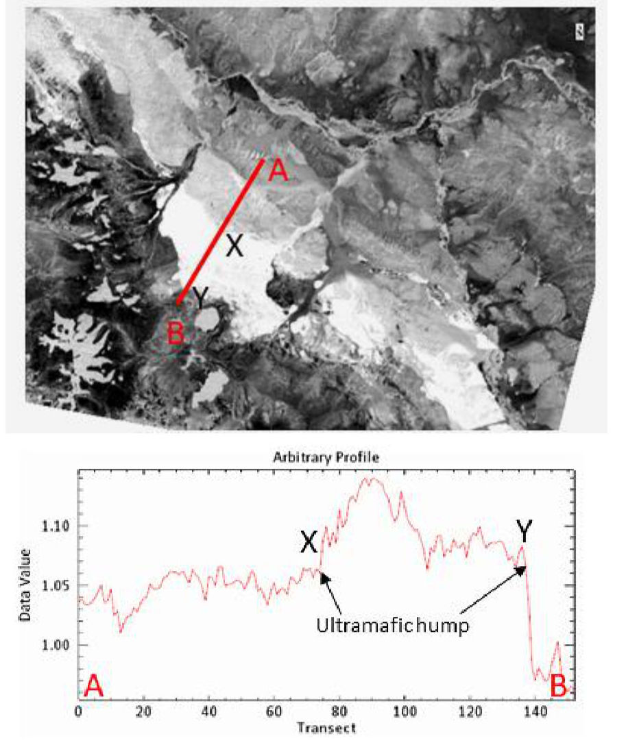
Figure 5.4a — ASTER mafic index (top panel) showing ultramafic units in bright white. The A–B transect profile (bottom panel) shows the sharp value jump across the lithological contact, demonstrating the index's ability to detect mineralogical boundaries. Source: Ghaste (2020), thesis Fig. 42.
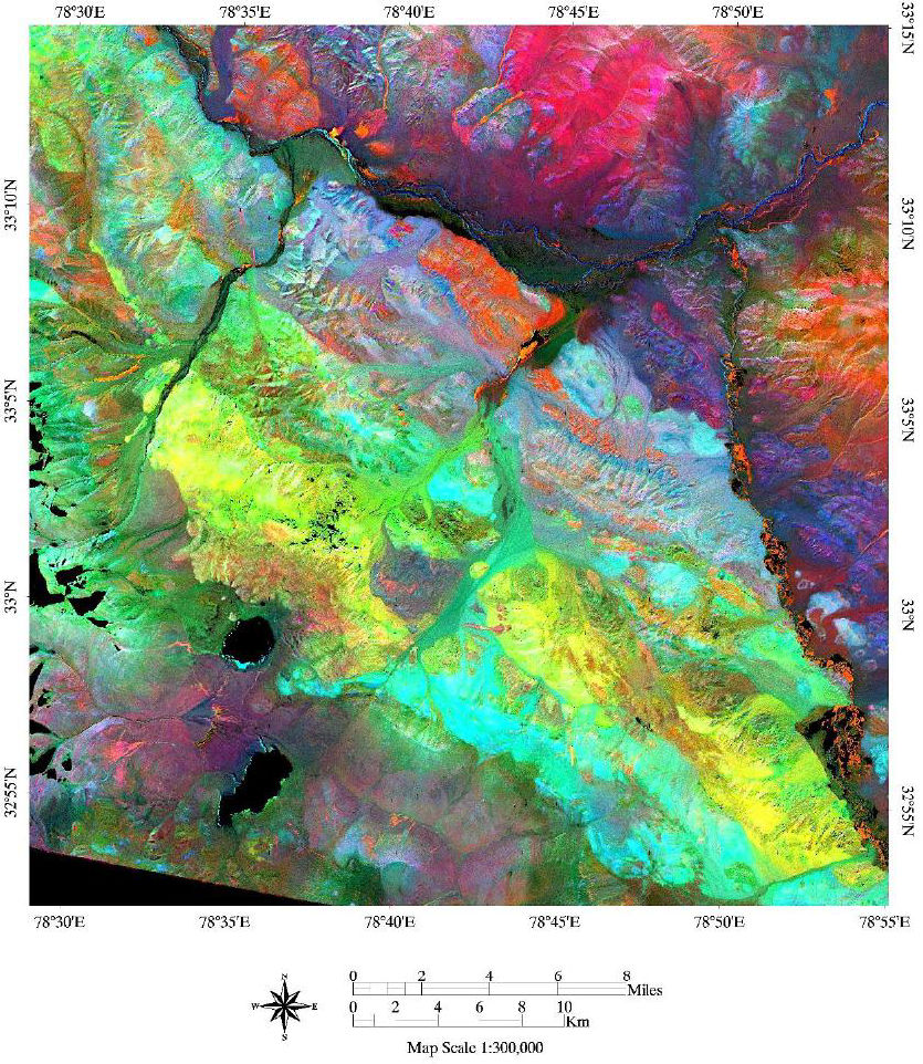
Figure 5.4b — ASTER serpentine index — false-colour composite of bands 3/1, 5/7, 5/3 (RGB). Serpentinised zones appear in yellow-green tones, revealing the internal pattern of serpentinisation within the ultramafic unit. Where the mafic index identifies where the ultramafic rocks are, the serpentine index reveals how altered they are. Source: Ghaste (2020), thesis Fig. 43.
Key Insight: Physical Meaning First
Every index should be understood in terms of the mineral physics it encodes before it is applied. The serpentine index works because serpentine minerals have a specific peak-trough contrast in the 2150–2280 nm range. If you are working in a different geological setting (e.g., carbonates, phyllic alteration), different band combinations are needed. Never copy index formulas without understanding their physical basis.
E) Supervised Classification Methods
Classification assigns every pixel in an image to one of a set of predefined geological classes based on its spectral properties. Supervised classification uses training data (ROIs) collected from pixels of known class identity to build decision rules. Three algorithms were applied to the ASTER SWIR data in the Nidar study.
Minimum Distance Classifier
The simplest geometrical classifier. For each class, a mean spectral vector is calculated from training pixels. An unknown pixel is assigned to the class whose mean vector is nearest in Euclidean distance in the spectral feature space. Think of it as finding the nearest city on a map, where each axis of the map is a different spectral band.
In the Nidar study, minimum distance was the most effective algorithm — producing classification outputs with minimal misclassification relative to the known field maps. This is because the major rock classes (dunite, peridotite, gabbro) are well separated in ASTER SWIR space, and the Euclidean distance metric was sufficient.
Maximum Likelihood Classifier
A probabilistic classifier that assumes each class has a Gaussian (normal) distribution in feature space. It assigns each pixel to the class with the highest probability of having generated that pixel's spectral values. A probability threshold of 0.15 was applied in the Nidar study — pixels with maximum class probability below 0.15 were left unclassified rather than forced into a class.
This threshold is geologically meaningful: pixels that sit between class distributions (e.g., mixed dunite-peridotite contacts) are genuinely ambiguous and should be flagged for field investigation rather than assigned with false confidence.
Spectral Angle Mapper (SAM)
SAM is the most powerful and physically motivated of the three classifiers for reflectance data. It represents each pixel's spectrum as a vector in n-dimensional space (where n = number of bands) and measures the angle between the pixel vector and a set of reference (endmember) vectors. A small angle means the pixel spectrum closely matches the reference; a large angle means it does not.
Figure 5.5 — Geometric concept of Spectral Angle Mapper (SAM). Each pixel spectrum is a vector in n-dimensional spectral space. SAM measures the angle θ between the target pixel vector and the reference (endmember) vector. Because this angle is independent of vector magnitude, SAM is insensitive to illumination variations — a critical advantage over distance-based classifiers.
SAM is particularly powerful because it is insensitive to illumination and albedo effects — two major sources of spectral variation in mountainous terrain. A pixel in shadow will have a lower magnitude vector than one in full sun, but the angle between them (if they are the same mineral) will be zero. This is a major advantage in high-relief terrain like Ladakh.
SAM Threshold Angles Used in the Nidar Study (ASTER, 9 SWIR bands)
| Class | Threshold Angle (radians) | Meaning |
|---|---|---|
| Gabbro | 0.065 | Broader class tolerance (more spectral heterogeneity) |
| Dunite | 0.050 | Moderate tolerance |
| Peridotite | 0.040 | Tighter class definition needed |
| Pillow Lava | 0.070 | Most variable (glassy groundmass, varying alteration) |
These thresholds were determined iteratively: starting from PPI-derived endmembers, the angle was tightened until mapped classes no longer "spilled" beyond their expected geographic extents as documented in existing field maps. Pixels outside all thresholds remain unclassified rather than being forced into a class.
Common Mistake
Using the same SAM threshold for every class and every scene. The optimal threshold varies by class (some rocks are more spectrally uniform than others) and by scene (atmospheric correction quality, topographic effects). Always iterate and validate thresholds against known field locations, not just against training ROIs.
Hyperspectral Analysis: The Power of Continuous Spectra
Everything in the traditional workflow improves with more spectral information. Hyperion provides hundreds of contiguous spectral channels, enabling a qualitatively different type of geological analysis — one that resembles the analysis a geochemist performs in a laboratory, now extended to the scale of a satellite scene.
Discrete vs Continuous Spectra: What Changes?
With Sentinel-2, you have 2 SWIR data points. With ASTER, you have 6. With Hyperion, you have over 170 contiguous samples across the same range. This matters because mineral absorption features have specific shapes — not just positions. A broad, asymmetric trough at 2290 nm tells a different story than a sharp, symmetric trough at the same position. With multispectral data, you can detect a feature is present; with hyperspectral data, you can characterise its shape.
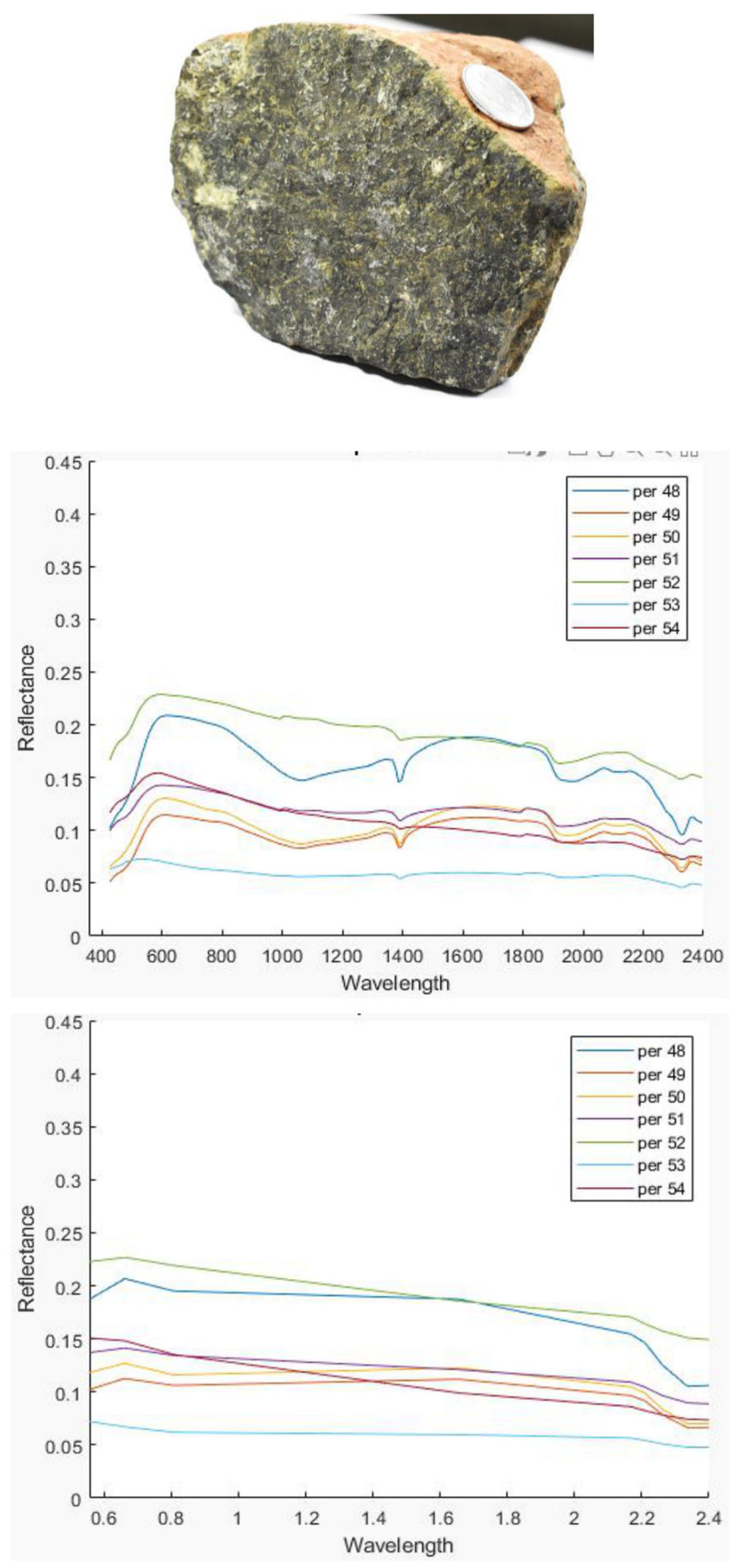
Figure 6.1 — The same peridotite sample seen at two different spectral resolutions. The continuous ASD field spectrum (top) — analogous to a Hyperion observation — fully resolves the Mg-OH absorption feature near 2300 nm. The same spectrum resampled to ASTER's 9 SWIR bands (bottom) captures the feature only as a coarse two-point depression. Sentinel-2's broad SWIR bands (not shown) would not resolve it at all. Spectral resolution determines whether a sensor detects, approximates, or fully resolves a mineralogical absorption feature. Source: Ghaste (2020).
Hyperion Preprocessing: Noise First
Hyperion data requires more preprocessing than multispectral data. With 200+ bands, noise accumulates and many bands are unreliable (particularly around atmospheric absorption windows at ~1400 and ~1900 nm). The standard workflow applies:
- Noisy band removal — bands dominated by water vapour absorption are excluded.
- FLAASH atmospheric correction — as described in Section 4.
- MNF (Minimum Noise Fraction) transform — separates signal from noise. MNF is a modified PCA that orders components by SNR rather than variance. The first MNF bands contain the most coherent signal; later ones are noise-dominated.
- PPI (Pixel Purity Index) — identifies the most spectrally pure pixels (candidate endmembers) by iteratively projecting n-dimensional data and counting extreme pixels.
- Endmember identification — inspect candidate endmember spectra in an n-D visualiser and match to known field spectra or library references.
Hyperion Band Indices Used in the Nidar Study
Three targeted indices were applied to the Hyperion image to map specific chemical signatures within the ultramafic terrain near Hanle:
High scores in the Mg-OH index indicate OH-altered and carbonate-bearing zones, normally concentrated in ultramafic rocks compared to volcano-sedimentary units. The ferrous index highlights zones of Fe²⁺-bearing mineralogy (olivine, pyroxene). Together, these three indices provide a chemical fingerprint of the alteration state within the ophiolite.
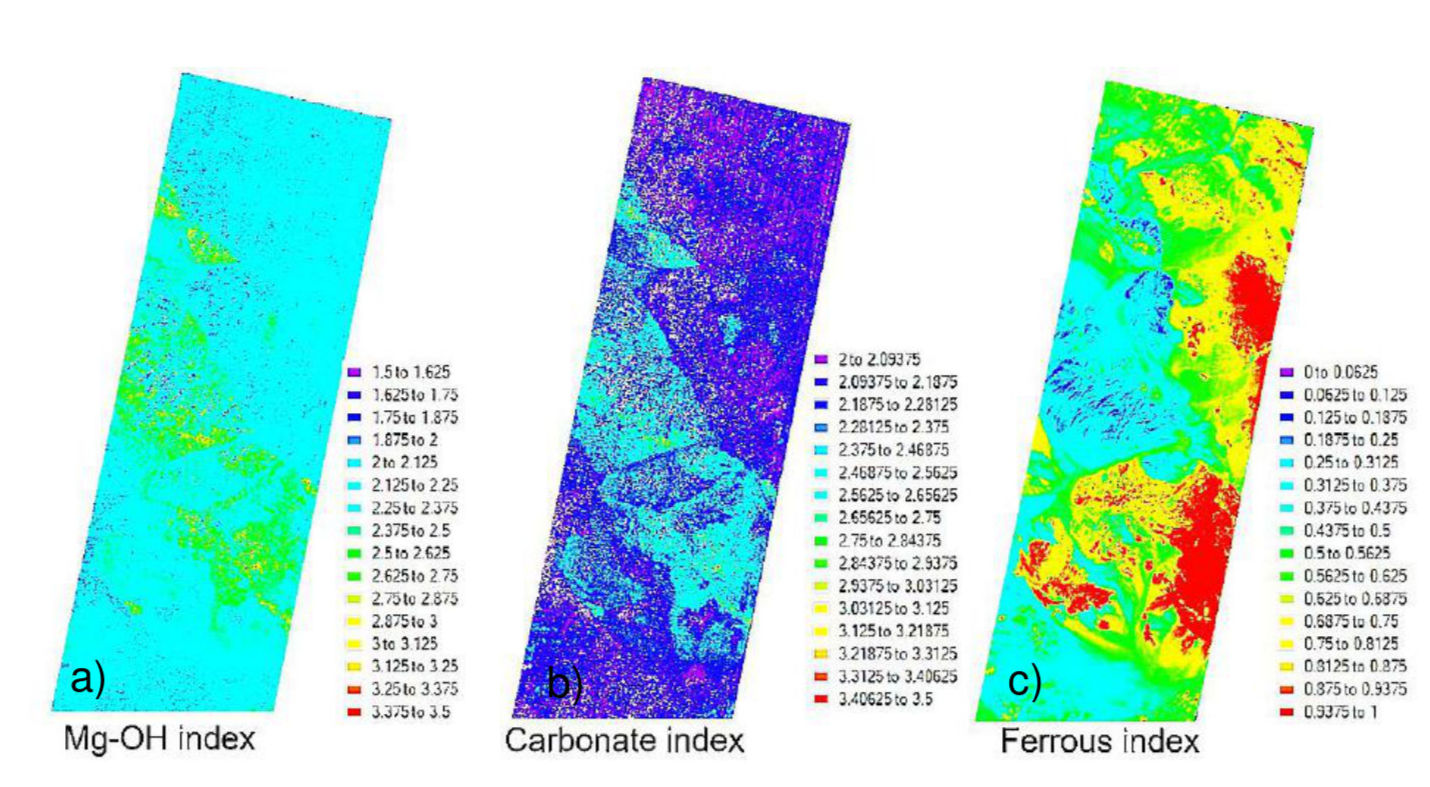
Figure 6.2 — Hyperion-derived mineral indices for the Hanle extension of the Nidar Ophiolite Complex. (a) Mg-OH Index — elevated values indicate serpentine-bearing ultramafics; (b) Carbonate Index — highlights hydrothermal carbonate veining associated with ocean-floor alteration; (c) Ferrous Index — distinguishes the iron-bearing mineralogy of fresh ultramafics from altered or oxidised facies. Source: Ghaste (2020), thesis Fig. 47.
Key Insight
The scientific value of hyperspectral data is not simply "more bands." It is the ability to characterise spectral curve shape — the geometry of absorption features — rather than just their presence. This enables mineral-specific mapping (e.g., distinguishing serpentine polymorphs like antigorite vs lizardite) that is physically impossible with multispectral data, regardless of classification algorithm sophistication.
AI-Based Geological Mapping: From Rules to Learning
Traditional remote sensing uses physics and expert knowledge to design features (ratios, indices) and decision rules (classifiers). Machine learning inverts this: instead of designing features manually, it learns them from labelled examples. This section explains how that transition works for geological mapping and where the physics-based and data-driven approaches complement each other.
Why Traditional Methods Have Limits
Classical methods like SAM and Maximum Likelihood work well when:
- Classes are spectrally distinct in the available bands.
- Training ROIs are clean and representative.
- The scene is spatially uniform enough that atmospheric correction is consistent.
They struggle when classes overlap spectrally (e.g., partially serpentinized peridotite vs fully serpentinized dunite), when spatial texture matters (e.g., banded ultramafics where the spatial pattern of alternating rock types is the signal), or when you want to simultaneously use many types of ancillary data (elevation, slope, curvature, published geological age). This is where machine learning adds value.
Feature Engineering: Building on Physics
The most powerful AI pipelines are not purely data-driven — they are physics-informed. Rather than feeding raw band values to a classifier, you construct a feature matrix that includes physically meaningful derived quantities:
Spectral bands
Individual ASTER/Sentinel/Hyperion band reflectances — provides baseline spectral information.
Band ratios & indices
Mafic index, serpentine index, Mg-OH index — encodes geochemical and mineralogical contrasts.
PCA components
Decorrelated variance components — often highlights subtle compositional gradients invisible in raw bands.
Terrain attributes
SRTM elevation, slope, aspect, curvature — geology is not random in topographic space; dunites and peridotites occupy structurally distinct positions.
Texture metrics
GLCM contrast, homogeneity, entropy — mafic and ultramafic units often have distinct roughness at the pixel scale due to differential weathering.
Multi-sensor fusion
Combined features from Sentinel-2 (spatial) + ASTER (mineralogical) + DEM (topographic) — the information in each is complementary, not redundant.
Machine Learning Classifiers for Geological Mapping
Random Forest (RF)
An ensemble of decision trees, each trained on a random subset of training samples and features. RF is robust to overfitting, handles high-dimensional feature spaces well, and provides feature importance scores — telling you which spectral or topographic variables most discriminate each class. This is the approach demonstrated in the Geonome Kalpa tutorial for Ladakh lithological classification.
Support Vector Machine (SVM)
Finds the optimal hyperplane separating classes in feature space. Effective when classes are small and well-separated. Can use non-linear kernels to handle complex spectral mixing. More sensitive to feature scaling than RF.
Convolutional Neural Networks (CNN)
When applied to hyperspectral cubes or image patches, CNNs can learn both spectral and spatial features simultaneously. Most powerful when training data is large and the spatial pattern of lithological units is informative. Requires more data and training infrastructure than RF or SVM.
Spectral-Spatial Deep Learning
Combines a 1D spectral branch (processing the full spectral curve at each pixel) with a 2D spatial branch (processing image texture around each pixel). State-of-the-art for hyperspectral classification when ground truth is available.
Physics-Based vs Data-Driven: A Structural Comparison
| Dimension | Physics-based (SAM, band ratios) | Data-driven (RF, CNN) |
|---|---|---|
| Interpretability | High — every decision has a physical explanation | Variable — RF gives feature importance; deep learning is opaque |
| Training data required | Minimal (only endmembers/ROIs) | Substantial (hundreds to thousands of labelled pixels per class) |
| Generalisation to new scenes | Good — physics is scene-independent | Can degrade if training and test scenes have different atmospheric/lighting conditions |
| Handling spectral overlap | Limited — angle/distance metrics struggle with mixed classes | Often better — nonlinear boundaries in feature space |
| Use of ancillary data | Limited — most methods work in spectral space only | Natural — features from any source can be added to the input matrix |
| Best use case | Initial mapping, small datasets, interpretable outputs, new geological settings | Large scenes, complex multi-class problems, operational workflows with stable training |
Validation Protocol: Non-Negotiable Steps
Training and validation ROIs must be spatially independent — not just different pixels from the same polygon. Use different outcrop locations for training and testing.
Report Producer's Accuracy, User's Accuracy, and F1-score for each class. Overall accuracy hides poor performance on rare classes (e.g., chromitite, pillow lava).
Do classified polygons make geological sense? Dunite bodies should be spatially contiguous, not scattered randomly. Gabbroic intrusions in peridotite are geologically expected; salt-and-pepper misclassification is not.
Compare against published geological maps (e.g., Buchs et al. 2018 for Nidar). Systematic disagreement should be investigated, not simply dismissed.
Common Mistake
Reporting a single overall accuracy figure (e.g., 87%) without per-class breakdown or spatial validation. A classifier that achieves high overall accuracy by correctly mapping abundant alluvium pixels while completely misclassifying rare dunite bodies is not useful for geological mapping. Always inspect the map, not just the numbers.
Case Study: Nidar Ophiolite Complex, Ladakh
This section ties together every concept and method from the tutorial through a real geological example. The Nidar Ophiolite Complex (NOC) is an obducted slab of oceanic lithosphere exposed in the Trans-Himalayan terrain of Ladakh, NW India. Its lithological diversity — dunite, peridotite, gabbro, pillow lava, pyroxenite — makes it an ideal test bench for multi-sensor satellite mapping.
Geological Setting
Ophiolites are fragments of ancient oceanic crust and upper mantle that have been thrust onto continental margins during tectonic collisions. The Nidar Ophiolite records the closure of the Neo-Tethys Ocean as the Indian subcontinent collided with Asia. From bottom to top (south to north in the NOC), the exposed section follows the classic ophiolite stratigraphy:
Plutonic Sequence (Mantle section)
- Dunite — >90% olivine, forms the base. Extremely prone to serpentinization (10–100% serpentinites observed). Key satellite signature: high reflectance at ASTER Band 4 (1.65 μm), diagnostic dip at ~2250 nm from serpentine weathering.
- Harzburgite / Peridotite — olivine + orthopyroxene ± clinopyroxene. Also serpentinized. Key signature: strong V-shaped Mg-OH trough at ~2300 nm, absorptions at 960, 1740, 1860, 2340, 2420 nm.
- Chromitite pods — dense chromite in ultramafic host. Satellite signature: nearly featureless, very dark.
Crustal Sequence (Intrusive and extrusive)
- Gabbro — plagioclase + clinopyroxene ± olivine. Forms small intrusive bodies in the mantle unit. Key signature: W-shaped double trough at 2200–2400 nm, lower overall reflectance than dunite in Band 4.
- Pyroxenite — orthopyroxene-dominated. Shows exsolution lamellae, indicating complex thermal history.
- Pillow Lava — extrusive basalt. Key signature: broad Fe²⁺ absorption near 900 nm, no strong SWIR features.
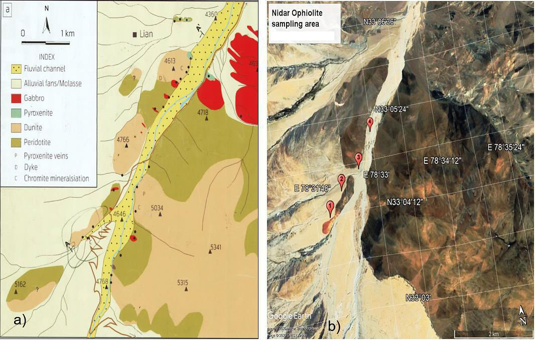
Figure 8.1 — The Nidar Ophiolite Complex study area. The from-south-to-north section through the complex reveals the plutonic sequence (dunite, peridotite, gabbro) succeeded by pillow lavas and overlying sedimentary units. Field sample collection points guided the selection of training regions of interest (ROIs) for all classifiers in this study. Source: Ghaste (2020), thesis Fig. 9.
Multi-Sensor Evidence Chain
The Nidar study was not solved by a single dataset. Each sensor contributed something the others could not:
Step 1: First-order separation
FCC (Band 11 red, Band 12 green, Band 8A blue) separates the mafic-ultramafic suite (pinkish brown) from sedimentary sequences (yellowish green). Dunite's dip at ~2250 nm in Band 12 provides its only clear Sentinel-2 signature. Gabbro and peridotite are not separable — too similar in limited SWIR.
Step 2: Lithological discrimination
FCC 7-4-2 separates dunite (bright green), peridotite (dark brown), gabbro (light greenish). Spectral profiles confirm V-shape (peridotite) vs W-shape (gabbro). SAM classification successfully maps dunite (cyan), peridotite (yellow), gabbro (red), pillow lava (magenta) with geologically consistent spatial distributions. Minimum distance classification matches best against field maps with minimal misclassification.
Step 3: Thermal confirmation
Emissivity profiles confirm the physics: peridotite (ultramafic) has higher emissivity at bands 10–12 and lower at 13–14. Gabbro (mafic) has the opposite trend. The mafic index (Band 12/13) cleanly delineates the ultramafic unit in bright white with sharp contacts. The thermal FCC (Band 13/10, 14/10, 13/12) shows gabbro in dark purple and peridotite/dunite in dark green.
Step 4: Serpentinization mapping
The serpentine index FCC (Band 3/1, 5/7, 5/3) highlights serpentinized peridotites and dunites in pale green to yellow. Peridotite and dunite are confirmed as the most serpentinized units (as expected from olivine content). Gabbro shows minimal serpentinization signature.
Step 5: Mineralogical refinement (Hanle area)
K-means unsupervised classification reveals 3 of 7 classes consistent with ultramafic groupings. Supervised SAM validates peridotite occurrence at Hanle (consistent with Duraiswami et al. 2014). Mg-OH and carbonate indices confirm OH-alteration and hydrothermal carbonate concentrated in ultramafics.
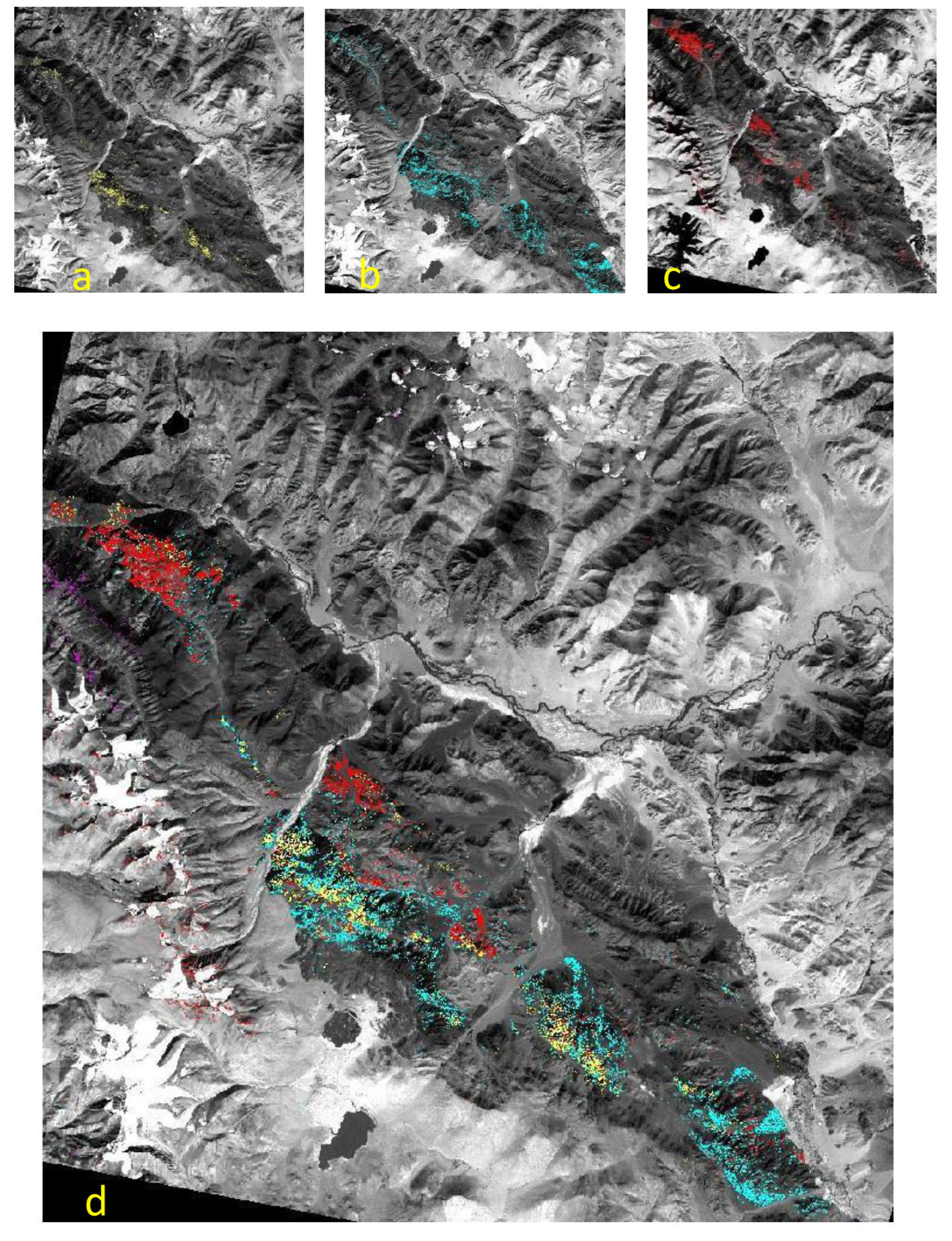
Figure 8.2 — ASTER Spectral Angle Mapper (SAM) classification of the Nidar Ophiolite Complex. (a) SAM classification for peridotite. (b) SAM classification for dunite. (c) SAM classification for gabbro. (d) SAM classification for pillow lava. Together with the mafic index (Fig. 5.4a), serpentine index (Fig. 5.4b), and published field geology, these classification products form a multi-line evidence stack — convergence between independent products gives confidence in the final lithological interpretation. Source: Ghaste (2020), thesis Fig. 38.
Key Geological Findings
- SAM classification on ASTER SWIR data successfully discriminated dunite, peridotite, gabbro, and pillow lava within the ophiolite suite.
- Peridotite and dunite are the most serpentinized units, validated by both spectral indices and thin section analysis showing mesh texture and serpentine veins around relict olivine.
- Gabbroic intrusions within the peridotite mantle unit are geologically expected and confirmed by image analysis — visible as isolated gabbro (red) pixels within the peridotite-dominated zone.
- Hyperion data extended the analysis eastward to Hanle, confirming peridotite presence far from the main Nidar Valley outcrops.
- ASTER is the most effective single sensor for regional lithological classification because of its unique combination of SWIR and TIR coverage.
Key Insight: Evidence Convergence
No single map product from any single sensor is the "answer." Confidence in a geological interpretation comes from convergence of independent evidence lines: spectral profiles, band indices, multiple classifiers, thermal emissivity, petrographic thin sections, and published field geology. When multiple independent methods agree on a boundary, you can trust it. When they disagree, that disagreement is itself a geological signal worth investigating.
Common Mistake
Reporting only the best-looking classification map without discussing where it agrees and disagrees with independent evidence. Geologically mixed zones (e.g., gabbroic intrusions in peridotite at the 30 m pixel scale) will produce systematic classification uncertainty. This is not a failure — it is a physically meaningful result reflecting real geological mixing.